!pip install matplotlib pandas pyarrow seaborn

import pandas as pd
import seaborn as sns
import matplotlib.pyplot as plt

plt.rcParams["font.family"] = "sans"
plt.rcParams["font.size"] = 8
sns.set_palette('muted')

Shot Metadata

This notebook contains a demonstration of plotting several of the summary statistics that accompany the shot metadata.

Firstly, we’re going to load all the shot data into a pandas dataframe:

summary = pd.read_parquet('https://mastapp.site/parquet/level2/shots')
summary = summary.loc[summary.shot_id <40000]
summary

	context	url	preshot_description	postshot_description	campaign	current_range	divertor_config	plasma_shape	commissioner	facility	...	cpf_vol_ipmax	cpf_vol_max	cpf_vol_truby	cpf_wmhd_ipmax	cpf_wmhd_max	cpf_wmhd_truby	cpf_zeff_ipmax	cpf_zeff_max	cpf_zeff_truby	cpf_zmag_efit
0	{'dcat': 'http://www.w3.org/ns/dcat#', 'dct': ...	s3://mast/level2/shots/11766.zarr	\nRELOAD 10232 PLASMA CONDITIONING SHOT FROM M4\n	\nGOOD PLASMA, RAN FINE. SL JOINT ALARMS RATHE...	M5	None	Conventional	None	None	MAST	...	8.088068	8.478948	NaN	9286.269388	14370.632	NaN	NaN	NaN	NaN	-0.011828
1	{'dcat': 'http://www.w3.org/ns/dcat#', 'dct': ...	s3://mast/level2/shots/11767.zarr	\nREPEAT\n	\nOK BUT LOST VERTICAL CONTROL - FA2 JUST DIED...	M5	None	Conventional	None	None	MAST	...	7.707199	8.559942	NaN	7343.788162	11461.490	NaN	NaN	NaN	NaN	-0.007570
2	{'dcat': 'http://www.w3.org/ns/dcat#', 'dct': ...	s3://mast/level2/shots/11768.zarr	\nSELECT ALL 4 FAS AND LOAD EFC SETTINGS FROM ...	\nOK. GOT FA4 BUT NOT FA3\n	M5	None	Conventional	None	None	MAST	...	8.300782	8.580827	NaN	10585.928086	12660.081	NaN	NaN	NaN	NaN	-0.011107
3	{'dcat': 'http://www.w3.org/ns/dcat#', 'dct': ...	s3://mast/level2/shots/11769.zarr	\nREPEAT, WITH TF RAISED TO 0.58.\n	\nSLIDING JOINT ALARMS A BIT LOWER. PLASMA OK.\n	M5	None	Conventional	None	None	MAST	...	8.112973	8.742647	NaN	8189.273726	12494.456	NaN	NaN	NaN	NaN	-0.008156
4	{'dcat': 'http://www.w3.org/ns/dcat#', 'dct': ...	s3://mast/level2/shots/11771.zarr	\nRELOADED 11769 AND SET UP PLASMA CURRENT FEE...	\nGOOD PLASMA F/B CONTROL. SLIDING JOINT ALARM...	M5	None	Conventional	None	None	MAST	...	7.978917	8.760519	NaN	8206.258460	12345.816	NaN	NaN	NaN	NaN	-0.008726
...	...	...	...	...	...	...	...	...	...	...	...	...	...	...	...	...	...	...	...	...	...
11276	{'dcat': 'http://www.w3.org/ns/dcat#', 'dct': ...	s3://mast/level2/shots/30467.zarr	\nRepeat with new neutron camera position.\ncH...	\nTwo times lower DD neutron rate than referen...	M9	700 kA	Conventional	Connected Double Null	None	MAST	...	9.029202	9.046394	NaN	49469.122469	52653.445	NaN	NaN	NaN	NaN	0.013202
11277	{'dcat': 'http://www.w3.org/ns/dcat#', 'dct': ...	s3://mast/level2/shots/30468.zarr	\nRepeat with new neutron camera position.\ncH...	\nGood beam.\nGood repeat.\n	M9	700 kA	Conventional	Lower Single Null	None	MAST	...	9.102411	9.107017	NaN	48516.962675	49382.133	NaN	NaN	NaN	NaN	0.012445
11278	{'dcat': 'http://www.w3.org/ns/dcat#', 'dct': ...	s3://mast/level2/shots/30469.zarr	\nRepeat with increased beam power (74 kV)\ncH...	\nGood shot. Modes present.\n	M9	700 kA	Conventional	Connected Double Null	None	MAST	...	8.988730	9.047923	NaN	47466.249616	49115.805	NaN	NaN	NaN	NaN	0.015299
11279	{'dcat': 'http://www.w3.org/ns/dcat#', 'dct': ...	s3://mast/level2/shots/30470.zarr	\nRepeat last using hydrogen in outboard and c...	\nNo HF gas.\n	M9	700 kA	Conventional	None	None	MAST	...	9.687049	10.055509	NaN	17290.432865	22310.516	NaN	NaN	NaN	NaN	0.015164
11280	{'dcat': 'http://www.w3.org/ns/dcat#', 'dct': ...	s3://mast/level2/shots/30471.zarr	\nThe last plasma:\nConvert to i/b Helios 1724...	\nGood shot.\n	M9	700 kA	Conventional	Lower Single Null	None	MAST	...	8.817559	9.283702	NaN	38063.582380	40906.090	NaN	NaN	NaN	NaN	0.014340

11281 rows × 290 columns

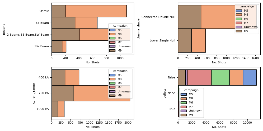
Summary Statistics About Shots

Let’s look at a summary of simple counts of different shot metadata.

fig, axes = plt.subplots(2, 2, figsize=(10, 5))
ax1, ax2, ax3, ax4 = axes.flatten()

sns.histplot(summary, y='heating', hue='campaign', multiple="stack", ax=ax1)
sns.histplot(summary, y='plasma_shape', hue='campaign', multiple="stack", ax=ax2)
sns.histplot(summary, y='current_range', hue='campaign', multiple="stack", ax=ax3)
sns.histplot(summary, y=summary.pellets.astype(str), hue='campaign', multiple="stack", ax=ax4)

for ax in axes.flatten():
    ax.set_xlabel('No. Shots')

plt.tight_layout()

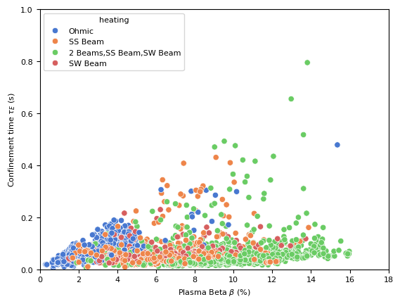
Plasma Beta (\(\beta\)) v.s Confinement Time (\(\tau_E\))

This plot can show how the efficiency of energy confinement varies with plasma pressure.

plt.figure()
sns.scatterplot(summary, y='cpf_tautot_max', x='cpf_betmhd_max', hue='heating')
plt.xlim(0, 18)
plt.ylim(0, 1)
plt.ylabel('Confinement time $\\tau_E$ (s)')
plt.xlabel('Plasma Beta $\\beta$ (%)')
plt.show()

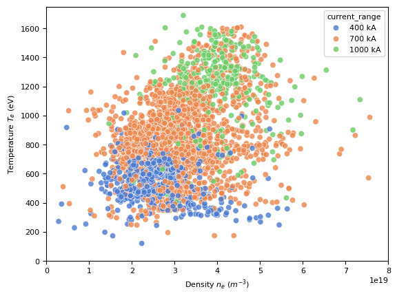
Plasma Temperature (\(T_e\)) vs. Plasma Density (\(n_e\))

This can reveal the relationship between temperature and density, which is critical for achieving the conditions necessary for fusion.

plt.figure()
sns.scatterplot(summary, y='cpf_te0_ipmax', x='cpf_ne0_ipmax', hue='current_range', alpha=0.8)
plt.xlim(0, .8e20)
plt.ylim(0, 1750)
plt.ylabel('Temperature $T_e$ (eV)')
plt.xlabel('Density $n_e$ ($m^{-3}$)')
plt.show()

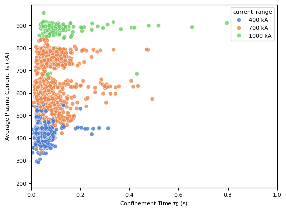
Plasma Current (\(I_p\)) vs. Confinement Time (\(\tau_E\))

This can indicate how the plasma current affects the confinement time, providing insights into stability and performance.

plt.figure()
sns.scatterplot(summary, y='cpf_ip_av', x='cpf_tautot_max', hue='current_range', alpha=0.8)
plt.xlim(0, 1)
plt.xlabel('Confinement Time $\\tau_E$ (s)')
plt.ylabel('Average Plasma Current  $I_p$ (kA)')
plt.show()