!pip install aiohttp matplotlib requests scipy "xarray[io]"
Show code cell output
Hide code cell output
Requirement already satisfied: aiohttp in /home/deploy/.local/lib/python3.8/site-packages (3.10.11)
Requirement already satisfied: matplotlib in /usr/lib/python3/dist-packages (3.1.2)
Requirement already satisfied: requests in /usr/lib/python3/dist-packages (2.22.0)
Requirement already satisfied: scipy in /home/deploy/.local/lib/python3.8/site-packages (1.10.1)
Requirement already satisfied: xarray[io] in /home/deploy/.local/lib/python3.8/site-packages (2023.1.0)
Requirement already satisfied: multidict<7.0,>=4.5 in /home/deploy/.local/lib/python3.8/site-packages (from aiohttp) (6.1.0)
Requirement already satisfied: aiosignal>=1.1.2 in /home/deploy/.local/lib/python3.8/site-packages (from aiohttp) (1.3.1)
Requirement already satisfied: aiohappyeyeballs>=2.3.0 in /home/deploy/.local/lib/python3.8/site-packages (from aiohttp) (2.4.4)
Requirement already satisfied: yarl<2.0,>=1.12.0 in /home/deploy/.local/lib/python3.8/site-packages (from aiohttp) (1.15.2)
Requirement already satisfied: async-timeout<6.0,>=4.0; python_version < "3.11" in /home/deploy/.local/lib/python3.8/site-packages (from aiohttp) (5.0.1)
Requirement already satisfied: frozenlist>=1.1.1 in /home/deploy/.local/lib/python3.8/site-packages (from aiohttp) (1.5.0)
Requirement already satisfied: attrs>=17.3.0 in /usr/lib/python3/dist-packages (from aiohttp) (19.3.0)
Requirement already satisfied: numpy<1.27.0,>=1.19.5 in /home/deploy/.local/lib/python3.8/site-packages (from scipy) (1.24.4)
Requirement already satisfied: pandas>=1.3 in /home/deploy/.local/lib/python3.8/site-packages (from xarray[io]) (2.0.3)
Requirement already satisfied: packaging>=21.3 in /usr/local/lib/python3.8/dist-packages (from xarray[io]) (24.1)
Requirement already satisfied: zarr; extra == "io" in /home/deploy/.local/lib/python3.8/site-packages (from xarray[io]) (2.16.1)
Requirement already satisfied: netCDF4; extra == "io" in /home/deploy/.local/lib/python3.8/site-packages (from xarray[io]) (1.7.2)
Requirement already satisfied: pydap; python_version < "3.10" and extra == "io" in /home/deploy/.local/lib/python3.8/site-packages (from xarray[io]) (3.4.1)
Requirement already satisfied: fsspec; extra == "io" in /home/deploy/.local/lib/python3.8/site-packages (from xarray[io]) (2024.10.0)
Requirement already satisfied: pooch; extra == "io" in /home/deploy/.local/lib/python3.8/site-packages (from xarray[io]) (1.8.2)
Requirement already satisfied: cftime; extra == "io" in /home/deploy/.local/lib/python3.8/site-packages (from xarray[io]) (1.6.4.post1)
Requirement already satisfied: h5netcdf; extra == "io" in /home/deploy/.local/lib/python3.8/site-packages (from xarray[io]) (1.1.0)
Requirement already satisfied: rasterio; extra == "io" in /home/deploy/.local/lib/python3.8/site-packages (from xarray[io]) (1.3.11)
Requirement already satisfied: cfgrib; extra == "io" in /home/deploy/.local/lib/python3.8/site-packages (from xarray[io]) (0.9.15.0)
Requirement already satisfied: typing-extensions>=4.1.0; python_version < "3.11" in /home/deploy/.local/lib/python3.8/site-packages (from multidict<7.0,>=4.5->aiohttp) (4.13.2)
Requirement already satisfied: idna>=2.0 in /usr/lib/python3/dist-packages (from yarl<2.0,>=1.12.0->aiohttp) (2.8)
Requirement already satisfied: propcache>=0.2.0 in /home/deploy/.local/lib/python3.8/site-packages (from yarl<2.0,>=1.12.0->aiohttp) (0.2.0)
Requirement already satisfied: python-dateutil>=2.8.2 in /home/deploy/.local/lib/python3.8/site-packages (from pandas>=1.3->xarray[io]) (2.9.0.post0)
Requirement already satisfied: tzdata>=2022.1 in /home/deploy/.local/lib/python3.8/site-packages (from pandas>=1.3->xarray[io]) (2025.2)
Requirement already satisfied: pytz>=2020.1 in /home/deploy/.local/lib/python3.8/site-packages (from pandas>=1.3->xarray[io]) (2025.2)
Requirement already satisfied: asciitree in /home/deploy/.local/lib/python3.8/site-packages (from zarr; extra == "io"->xarray[io]) (0.3.3)
Requirement already satisfied: fasteners in /home/deploy/.local/lib/python3.8/site-packages (from zarr; extra == "io"->xarray[io]) (0.19)
Requirement already satisfied: numcodecs>=0.10.0 in /home/deploy/.local/lib/python3.8/site-packages (from zarr; extra == "io"->xarray[io]) (0.12.1)
Requirement already satisfied: certifi in /usr/lib/python3/dist-packages (from netCDF4; extra == "io"->xarray[io]) (2019.11.28)
Requirement already satisfied: docopt in /usr/lib/python3/dist-packages (from pydap; python_version < "3.10" and extra == "io"->xarray[io]) (0.6.2)
Requirement already satisfied: six>=1.4.0 in /usr/lib/python3/dist-packages (from pydap; python_version < "3.10" and extra == "io"->xarray[io]) (1.14.0)
Requirement already satisfied: beautifulsoup4 in /home/deploy/.local/lib/python3.8/site-packages (from pydap; python_version < "3.10" and extra == "io"->xarray[io]) (4.13.4)
Requirement already satisfied: Jinja2 in /usr/local/lib/python3.8/dist-packages (from pydap; python_version < "3.10" and extra == "io"->xarray[io]) (3.1.4)
Requirement already satisfied: Webob in /home/deploy/.local/lib/python3.8/site-packages (from pydap; python_version < "3.10" and extra == "io"->xarray[io]) (1.8.9)
Requirement already satisfied: platformdirs>=2.5.0 in /home/deploy/.local/lib/python3.8/site-packages (from pooch; extra == "io"->xarray[io]) (4.3.6)
Requirement already satisfied: h5py in /home/deploy/.local/lib/python3.8/site-packages (from h5netcdf; extra == "io"->xarray[io]) (3.11.0)
Requirement already satisfied: importlib-metadata; python_version < "3.10" in /usr/lib/python3/dist-packages (from rasterio; extra == "io"->xarray[io]) (1.5.0)
Requirement already satisfied: affine in /home/deploy/.local/lib/python3.8/site-packages (from rasterio; extra == "io"->xarray[io]) (2.4.0)
Requirement already satisfied: setuptools in /usr/lib/python3/dist-packages (from rasterio; extra == "io"->xarray[io]) (45.2.0)
Requirement already satisfied: click>=4.0 in /usr/lib/python3/dist-packages (from rasterio; extra == "io"->xarray[io]) (7.0)
Requirement already satisfied: cligj>=0.5 in /home/deploy/.local/lib/python3.8/site-packages (from rasterio; extra == "io"->xarray[io]) (0.7.2)
Requirement already satisfied: click-plugins in /home/deploy/.local/lib/python3.8/site-packages (from rasterio; extra == "io"->xarray[io]) (1.1.1.2)
Requirement already satisfied: snuggs>=1.4.1 in /home/deploy/.local/lib/python3.8/site-packages (from rasterio; extra == "io"->xarray[io]) (1.4.7)
Requirement already satisfied: eccodes>=0.9.8 in /home/deploy/.local/lib/python3.8/site-packages (from cfgrib; extra == "io"->xarray[io]) (2.42.0)
Requirement already satisfied: soupsieve>1.2 in /home/deploy/.local/lib/python3.8/site-packages (from beautifulsoup4->pydap; python_version < "3.10" and extra == "io"->xarray[io]) (2.7)
Requirement already satisfied: MarkupSafe>=2.0 in /usr/local/lib/python3.8/dist-packages (from Jinja2->pydap; python_version < "3.10" and extra == "io"->xarray[io]) (2.1.5)
Requirement already satisfied: pyparsing>=2.1.6 in /usr/lib/python3/dist-packages (from snuggs>=1.4.1->rasterio; extra == "io"->xarray[io]) (2.4.6)
Requirement already satisfied: cffi in /home/deploy/.local/lib/python3.8/site-packages (from eccodes>=0.9.8->cfgrib; extra == "io"->xarray[io]) (1.17.1)
Requirement already satisfied: findlibs in /home/deploy/.local/lib/python3.8/site-packages (from eccodes>=0.9.8->cfgrib; extra == "io"->xarray[io]) (0.1.1)
Requirement already satisfied: pycparser in /home/deploy/.local/lib/python3.8/site-packages (from cffi->eccodes>=0.9.8->cfgrib; extra == "io"->xarray[io]) (2.22)
import matplotlib.pyplot as plt
import numpy as np
import requests
import xarray as xr
from matplotlib.colors import LogNorm
from scipy.signal import stft

plt.rcParams["font.family"] = "sans"
plt.rcParams["font.size"] = 8
Level 1 Data#
This notebook contains example plots of data from different diagnostics across MAST without any preprocessing, interpolation, calibration, cropping, etc… applied to the dataset. Data in level 1 are supplied under the original names used during the time of MAST’s operation. This dataset contains all shots that could be pulled from the MAST archive, including instrument calibration and testing shots.
First we need to find the url to a particular shot. Here we are going to use shot 30421 as an example.
shot_data = requests.get("https://mastapp.site/json/shots/30421").json()
endpoint, url = shot_data["endpoint_url"], shot_data["url"]
shot_url = url.replace("s3:/", endpoint)
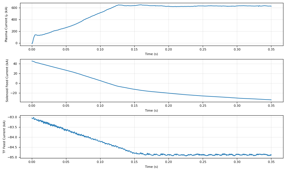
Plasma Current Data#
Data from the amc source contains
Plasma Current (\(I_p\)): Flows within the plasma, providing initial heating and contributing to the poloidal magnetic field for confinement and stability.
PF Coil Currents: Control the poloidal magnetic field, allowing for plasma shaping, vertical stability, and edge magnetic configuration control.
TF Coil Currents: Generate the strong toroidal magnetic field necessary for primary plasma confinement.
dataset = xr.open_zarr(shot_url, group='amc')
dataset = dataset.isel(time=(dataset.time > 0) & (dataset.time < .35))
fig, axes = plt.subplots(3, 1, figsize=(10, 6))
ax1, ax2, ax3 = axes.flatten()

ax1.plot(dataset['time'], dataset['plasma_current'])
ax1.set_xlabel('Time (s)')
ax1.set_ylabel('Plasma Current $I_p$ (kA)')

ax2.plot(dataset['time'], dataset['sol_current'])
ax2.set_xlabel('Time (s)')
ax2.set_ylabel('Solenoid Feed Current (kA)')

ax3.plot(dataset['time'], dataset['tf_current'])
ax3.set_xlabel('Time (s)')
ax3.set_ylabel('TF Feed Current (kA)')

for ax in axes:
    ax.grid(alpha=0.3)

plt.tight_layout()
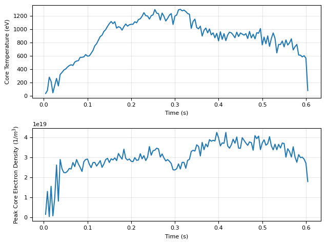
Thompson Scattering Data#
ayc source holds the Thomspon Scattering data at the core. Thomson scattering diagnostics provide accurate measurements of electron temperature and density.
dataset = xr.open_zarr(shot_url, group='ayc')
dataset = dataset[['te_core', 'ne_core']].dropna(dim='time')
fig, axes = plt.subplots(2,1)
ax1, ax2 = axes

ax1.plot(dataset['time'], dataset['te_core'])
ax1.set_xlabel('Time (s)')
ax1.set_ylabel('Core Temperature (eV)')

ax2.plot(dataset['time'], dataset['ne_core'])
ax2.set_xlabel('Time (s)')
ax2.set_ylabel('Peak Core Electron Density ($1 / m^3$)')

for ax in axes:
    ax.grid(alpha=0.3)

plt.tight_layout()
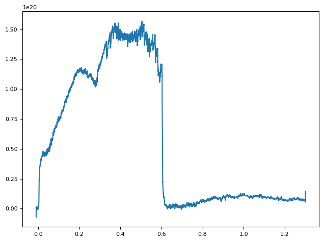
CO2 Interferometers#
CO2 interferometers (ane) are used to measure the electron density in the plasma. By measuring the phase shift of the laser beam as it passes through the plasma, the electron density can be inferred with high precision.
dataset = xr.open_zarr(shot_url, group='ane')
dataset
<xarray.Dataset> Size: 524kB
Dimensions:        (time: 32768)
Coordinates:
  * time           (time) float32 131kB -0.01 -0.00996 -0.00992 ... 1.301 1.301
Data variables:
    co2            (time) float32 131kB ...
    density        (time) float32 131kB ...
    hene           (time) float32 131kB ...
    passnumber     float32 4B ...
    status         float32 4B ...
    status_detail  float32 4B ...
    version        float32 4B ...
Attributes:
    description:  CO2 Interferometry
    file_name:    ane0304.21
    format:       IDA3
    mds_name:     None
    name:         ane
    quality:      Not Checked
    shot_id:      30421
    signal_type:  Analysed
    source:       ane
    uda_name:     ANE
    uuid:         825a1eac-b024-59a1-a792-326970dd47ec
version: 0- time: 32768
- time(time)float32-0.01 -0.00996 ... 1.301 1.301
- units :
- s
array([-0.01   , -0.00996, -0.00992, ...,  1.3006 ,  1.30064,  1.30068],
      shape=(32768,), dtype=float32)
- co2(time)float32...
- description :
- integrated electron density determined from co2 laser interference fringes
- dims :
- ['time']
- file_name :
- None
- format :
- None
- label :
- m^-2
- mds_name :
- \TOP.ANALYSED.ANE:CO2
- name :
- ane/co2
- quality :
- Not Checked
- rank :
- 1
- shape :
- [32768]
- shot_id :
- 30421
- signal_type :
- Analysed
- source :
- ane
- time_index :
- 0
- uda_name :
- ANE_CO2
- units :
- 1 / m ** 2
- uuid :
- 751982c7-2043-5cbb-8ccc-b76068364aab
- version :
- 0
[32768 values with dtype=float32]
- density(time)float32...
- description :
- integrated electron density including vibration correction
- dims :
- ['time']
- file_name :
- None
- format :
- None
- label :
- m^-2
- mds_name :
- \TOP.ANALYSED.ANE:DENSITY
- name :
- ane/density
- quality :
- Not Checked
- rank :
- 1
- shape :
- [32768]
- shot_id :
- 30421
- signal_type :
- Analysed
- source :
- ane
- time_index :
- 0
- uda_name :
- ANE_DENSITY
- units :
- 1 / m ** 2
- uuid :
- 4873688b-0fd0-53f3-9251-223cbbd963df
- version :
- 0
[32768 values with dtype=float32]
- hene(time)float32...
- description :
- electron density from HeNe fringes correspondes to vibrations in interferometer
- dims :
- ['time']
- file_name :
- None
- format :
- None
- label :
- m^-2
- mds_name :
- \TOP.ANALYSED.ANE:HENE
- name :
- ane/hene
- quality :
- Not Checked
- rank :
- 1
- shape :
- [32768]
- shot_id :
- 30421
- signal_type :
- Analysed
- source :
- ane
- time_index :
- 0
- uda_name :
- ANE_HENE
- units :
- 1 / m ** 2
- uuid :
- d2ed2ea0-62fd-575c-8c33-797d87cc162d
- version :
- 0
[32768 values with dtype=float32]
- passnumber()float32...
- description :
- Pass number of data
- dims :
- []
- file_name :
- None
- format :
- None
- label :
- Passno
- mds_name :
- \TOP.ANALYSED.ANE:PASSNUMBER
- name :
- ane/passnumber
- quality :
- Not Checked
- rank :
- 1
- shape :
- [1]
- shot_id :
- 30421
- signal_type :
- Analysed
- source :
- ane
- time_index :
- 0
- uda_name :
- ANE_PASSNUMBER
- units :
- uuid :
- 42c81c4d-b2da-5528-b58c-3c7dc44b4e8e
- version :
- 0
[1 values with dtype=float32]
- status()float32...
- description :
- status flag
- dims :
- []
- file_name :
- None
- format :
- None
- label :
- Status
- mds_name :
- \TOP.ANALYSED.ANE:STATUS
- name :
- ane/status
- quality :
- Not Checked
- rank :
- 1
- shape :
- [1]
- shot_id :
- 30421
- signal_type :
- Analysed
- source :
- ane
- time_index :
- 0
- uda_name :
- ANE_STATUS
- units :
- uuid :
- 91dff3cc-6060-5a7f-a69c-93c5d1167cdb
- version :
- 0
[1 values with dtype=float32]
- status_detail()float32...
- description :
- status detail
- dims :
- []
- file_name :
- None
- format :
- None
- label :
- status_detail
- mds_name :
- \TOP.ANALYSED.ANE.STATUS_:DETAIL
- name :
- ane/status_detail
- quality :
- Not Checked
- rank :
- 1
- shape :
- [1]
- shot_id :
- 30421
- signal_type :
- Analysed
- source :
- ane
- time_index :
- 0
- uda_name :
- ANE_STATUS_DETAIL
- units :
- uuid :
- d8d3709d-f229-5334-a0cb-a6c7b8eeb57f
- version :
- 0
[1 values with dtype=float32]
- version()float32...
- description :
- version of analysis code
- dims :
- []
- file_name :
- None
- format :
- None
- label :
- Version
- mds_name :
- \TOP.ANALYSED.ANE:VERSION
- name :
- ane/version
- quality :
- Not Checked
- rank :
- 1
- shape :
- [1]
- shot_id :
- 30421
- signal_type :
- Analysed
- source :
- ane
- time_index :
- 0
- uda_name :
- ANE_VERSION
- units :
- uuid :
- b16f44e9-8674-584a-9390-6abf21fd2636
- version :
- 0
[1 values with dtype=float32]
- timePandasIndex
PandasIndex(Index([-0.009999999776482582, -0.009959999471902847, -0.009920000098645687,
       -0.009879999794065952, -0.009839999489486217, -0.009800000116229057,
       -0.009759999811649323, -0.009719999507069588, -0.009680000133812428,
       -0.009639999829232693,
       ...
           1.300320029258728,    1.3003599643707275,    1.3004000186920166,
          1.3004399538040161,    1.3004800081253052,    1.3005199432373047,
          1.3005599975585938,    1.3005999326705933,    1.3006399869918823,
          1.3006799221038818],
      dtype='float32', name='time', length=32768))
- description :
- CO2 Interferometry
- file_name :
- ane0304.21
- format :
- IDA3
- mds_name :
- None
- name :
- ane
- quality :
- Not Checked
- shot_id :
- 30421
- signal_type :
- Analysed
- source :
- ane
- uda_name :
- ANE
- uuid :
- 825a1eac-b024-59a1-a792-326970dd47ec
- version :
- 0
dataset = xr.open_zarr(shot_url, group='ane')
plt.plot(dataset['time'], dataset['density'])
ax.set_xlabel('Time (s)')
ax.set_ylabel('Integrated Electron Density ($1 / m^2$)')
ax.grid(alpha=0.3)

plt.tight_layout()
Equillibrium Reconstruction Data#
The source efm contains data from EFIT. EFIT is a computational tool used to reconstruct the magnetic equilibrium configuration of the plasma in a tokamak. It calculates the shape and position of the plasma, as well as the distribution of the current and pressure within it, based on magnetic measurements.
dataset = xr.open_zarr(shot_url, group='efm')
dataset
<xarray.Dataset> Size: 8MB
Dimensions:            (time: 120, psi_norm: 65, n_iterations: 10,
                        fcoil_seg_n: 938, fcoil_n: 101, ffprime_coefs_n: 2,
                        mag_probe_n: 78, psi_loop_n: 46, r: 65, z: 65,
                        profile_r: 129, lcfs_coords: 139, limiter_n: 37,
                        pprime_coefs_n: 2, profile_z: 65)
Coordinates: (12/13)
  * fcoil_n            (fcoil_n) float32 404B 0.0 1.0 2.0 ... 98.0 99.0 100.0
  * ffprime_coefs_n    (ffprime_coefs_n) float32 8B 0.0 1.0
  * lcfs_coords        (lcfs_coords) float32 556B 0.0 1.0 2.0 ... 137.0 138.0
  * mag_probe_n        (mag_probe_n) float32 312B 0.0 1.0 2.0 ... 75.0 76.0 77.0
  * n_iterations       (n_iterations) float32 40B 0.0 1.0 2.0 ... 7.0 8.0 9.0
  * pprime_coefs_n     (pprime_coefs_n) float32 8B 0.0 1.0
    ...                 ...
  * profile_z          (profile_z) float32 260B -2.0 -1.938 -1.875 ... 1.938 2.0
  * psi_loop_n         (psi_loop_n) float32 184B 0.0 1.0 2.0 ... 43.0 44.0 45.0
  * psi_norm           (psi_norm) float32 260B 0.0 0.01562 ... 0.9844 1.0
  * r                  (r) float32 260B 0.06 0.09031 0.1206 ... 1.939 1.97 2.0
  * time               (time) float32 480B -0.05 -0.045 -0.04 ... 0.56 0.565 0.6
  * z                  (z) float32 260B -2.0 -1.938 -1.875 ... 1.875 1.938 2.0
Dimensions without coordinates: fcoil_seg_n, limiter_n
Data variables: (12/151)
    all_times          (time) float32 480B ...
    areap_c            (time, psi_norm) float32 31kB ...
    betan              (time) float32 480B ...
    betap              (time) float32 480B ...
    betapd             (time) float32 480B ...
    betat              (time) float32 480B ...
    ...                 ...
    wpol               (time) float32 480B ...
    xpoint1_rc         (time) float32 480B ...
    xpoint1_zc         (time) float32 480B ...
    xpoint2_rc         (time) float32 480B ...
    xpoint2_zc         (time) float32 480B ...
    zbdry              (time) float32 480B ...
Attributes:
    description:  Basic EFIT
    file_name:    efm0304.21
    format:       IDA3
    mds_name:     None
    name:         efm
    quality:      Not Checked
    shot_id:      30421
    signal_type:  Analysed
    source:       efm
    uda_name:     EFM
    uuid:         e75f0185-8b80-58f7-a1dd-5f7fc4659a12
version: 0- time: 120
- psi_norm: 65
- n_iterations: 10
- fcoil_seg_n: 938
- fcoil_n: 101
- ffprime_coefs_n: 2
- mag_probe_n: 78
- psi_loop_n: 46
- r: 65
- z: 65
- profile_r: 129
- lcfs_coords: 139
- limiter_n: 37
- pprime_coefs_n: 2
- profile_z: 65
- fcoil_n(fcoil_n)float320.0 1.0 2.0 3.0 ... 98.0 99.0 100.0
- units :
array([ 0., 1., 2., 3., 4., 5., 6., 7., 8., 9., 10., 11., 12., 13., 14., 15., 16., 17., 18., 19., 20., 21., 22., 23., 24., 25., 26., 27., 28., 29., 30., 31., 32., 33., 34., 35., 36., 37., 38., 39., 40., 41., 42., 43., 44., 45., 46., 47., 48., 49., 50., 51., 52., 53., 54., 55., 56., 57., 58., 59., 60., 61., 62., 63., 64., 65., 66., 67., 68., 69., 70., 71., 72., 73., 74., 75., 76., 77., 78., 79., 80., 81., 82., 83., 84., 85., 86., 87., 88., 89., 90., 91., 92., 93., 94., 95., 96., 97., 98., 99., 100.], dtype=float32) - ffprime_coefs_n(ffprime_coefs_n)float320.0 1.0
- units :
array([0., 1.], dtype=float32)
- lcfs_coords(lcfs_coords)float320.0 1.0 2.0 ... 136.0 137.0 138.0
- units :
array([ 0., 1., 2., 3., 4., 5., 6., 7., 8., 9., 10., 11., 12., 13., 14., 15., 16., 17., 18., 19., 20., 21., 22., 23., 24., 25., 26., 27., 28., 29., 30., 31., 32., 33., 34., 35., 36., 37., 38., 39., 40., 41., 42., 43., 44., 45., 46., 47., 48., 49., 50., 51., 52., 53., 54., 55., 56., 57., 58., 59., 60., 61., 62., 63., 64., 65., 66., 67., 68., 69., 70., 71., 72., 73., 74., 75., 76., 77., 78., 79., 80., 81., 82., 83., 84., 85., 86., 87., 88., 89., 90., 91., 92., 93., 94., 95., 96., 97., 98., 99., 100., 101., 102., 103., 104., 105., 106., 107., 108., 109., 110., 111., 112., 113., 114., 115., 116., 117., 118., 119., 120., 121., 122., 123., 124., 125., 126., 127., 128., 129., 130., 131., 132., 133., 134., 135., 136., 137., 138.], dtype=float32) - mag_probe_n(mag_probe_n)float320.0 1.0 2.0 3.0 ... 75.0 76.0 77.0
- units :
array([ 0., 1., 2., 3., 4., 5., 6., 7., 8., 9., 10., 11., 12., 13., 14., 15., 16., 17., 18., 19., 20., 21., 22., 23., 24., 25., 26., 27., 28., 29., 30., 31., 32., 33., 34., 35., 36., 37., 38., 39., 40., 41., 42., 43., 44., 45., 46., 47., 48., 49., 50., 51., 52., 53., 54., 55., 56., 57., 58., 59., 60., 61., 62., 63., 64., 65., 66., 67., 68., 69., 70., 71., 72., 73., 74., 75., 76., 77.], dtype=float32) - n_iterations(n_iterations)float320.0 1.0 2.0 3.0 ... 6.0 7.0 8.0 9.0
- units :
array([0., 1., 2., 3., 4., 5., 6., 7., 8., 9.], dtype=float32)
- pprime_coefs_n(pprime_coefs_n)float320.0 1.0
- units :
array([0., 1.], dtype=float32)
- profile_r(profile_r)float320.0 0.01562 0.03125 ... 1.97 2.0
- units :
array([0. , 0.015625, 0.03125 , 0.046875, 0.06 , 0.0625 , 0.078125, 0.090312, 0.09375 , 0.109375, 0.120625, 0.125 , 0.140625, 0.150937, 0.15625 , 0.171875, 0.18125 , 0.1875 , 0.203125, 0.211563, 0.21875 , 0.234375, 0.241875, 0.25 , 0.265625, 0.272188, 0.28125 , 0.296875, 0.3025 , 0.3125 , 0.328125, 0.332813, 0.34375 , 0.359375, 0.363125, 0.375 , 0.390625, 0.393438, 0.40625 , 0.421875, 0.42375 , 0.4375 , 0.453125, 0.454063, 0.46875 , 0.484375, 0.5 , 0.514687, 0.515625, 0.53125 , 0.545 , 0.546875, 0.5625 , 0.575312, 0.578125, 0.59375 , 0.605625, 0.609375, 0.625 , 0.635938, 0.640625, 0.65625 , 0.66625 , 0.671875, 0.6875 , 0.696563, 0.703125, 0.71875 , 0.726875, 0.734375, 0.75 , 0.757188, 0.765625, 0.78125 , 0.7875 , 0.796875, 0.8125 , 0.817813, 0.828125, 0.84375 , 0.848125, 0.859375, 0.875 , 0.878438, 0.890625, 0.90625 , 0.90875 , 0.921875, 0.9375 , 0.939063, 0.953125, 0.96875 , 0.969375, 0.984375, 0.999688, 1. , 1.03 , 1.060313, 1.090625, 1.120937, 1.15125 , 1.181562, 1.211875, 1.242188, 1.2725 , 1.302812, 1.333125, 1.363438, 1.39375 , 1.424062, 1.454375, 1.484687, 1.515 , 1.545313, 1.575625, 1.605937, 1.63625 , 1.666562, 1.696875, 1.727188, 1.7575 , 1.787812, 1.818125, 1.848438, 1.87875 , 1.909063, 1.939375, 1.969687, 2. ], dtype=float32) - profile_z(profile_z)float32-2.0 -1.938 -1.875 ... 1.938 2.0
- units :
- m
array([-2. , -1.9375, -1.875 , -1.8125, -1.75 , -1.6875, -1.625 , -1.5625, -1.5 , -1.4375, -1.375 , -1.3125, -1.25 , -1.1875, -1.125 , -1.0625, -1. , -0.9375, -0.875 , -0.8125, -0.75 , -0.6875, -0.625 , -0.5625, -0.5 , -0.4375, -0.375 , -0.3125, -0.25 , -0.1875, -0.125 , -0.0625, 0. , 0.0625, 0.125 , 0.1875, 0.25 , 0.3125, 0.375 , 0.4375, 0.5 , 0.5625, 0.625 , 0.6875, 0.75 , 0.8125, 0.875 , 0.9375, 1. , 1.0625, 1.125 , 1.1875, 1.25 , 1.3125, 1.375 , 1.4375, 1.5 , 1.5625, 1.625 , 1.6875, 1.75 , 1.8125, 1.875 , 1.9375, 2. ], dtype=float32) - psi_loop_n(psi_loop_n)float320.0 1.0 2.0 3.0 ... 43.0 44.0 45.0
- units :
array([ 0., 1., 2., 3., 4., 5., 6., 7., 8., 9., 10., 11., 12., 13., 14., 15., 16., 17., 18., 19., 20., 21., 22., 23., 24., 25., 26., 27., 28., 29., 30., 31., 32., 33., 34., 35., 36., 37., 38., 39., 40., 41., 42., 43., 44., 45.], dtype=float32) - psi_norm(psi_norm)float320.0 0.01562 0.03125 ... 0.9844 1.0
- units :
array([0. , 0.015625, 0.03125 , 0.046875, 0.0625 , 0.078125, 0.09375 , 0.109375, 0.125 , 0.140625, 0.15625 , 0.171875, 0.1875 , 0.203125, 0.21875 , 0.234375, 0.25 , 0.265625, 0.28125 , 0.296875, 0.3125 , 0.328125, 0.34375 , 0.359375, 0.375 , 0.390625, 0.40625 , 0.421875, 0.4375 , 0.453125, 0.46875 , 0.484375, 0.5 , 0.515625, 0.53125 , 0.546875, 0.5625 , 0.578125, 0.59375 , 0.609375, 0.625 , 0.640625, 0.65625 , 0.671875, 0.6875 , 0.703125, 0.71875 , 0.734375, 0.75 , 0.765625, 0.78125 , 0.796875, 0.8125 , 0.828125, 0.84375 , 0.859375, 0.875 , 0.890625, 0.90625 , 0.921875, 0.9375 , 0.953125, 0.96875 , 0.984375, 1. ], dtype=float32) - r(r)float320.06 0.09031 0.1206 ... 1.97 2.0
- units :
- m
array([0.06 , 0.090312, 0.120625, 0.150937, 0.18125 , 0.211563, 0.241875, 0.272188, 0.3025 , 0.332813, 0.363125, 0.393438, 0.42375 , 0.454063, 0.484375, 0.514687, 0.545 , 0.575312, 0.605625, 0.635938, 0.66625 , 0.696563, 0.726875, 0.757188, 0.7875 , 0.817813, 0.848125, 0.878438, 0.90875 , 0.939063, 0.969375, 0.999688, 1.03 , 1.060313, 1.090625, 1.120937, 1.15125 , 1.181562, 1.211875, 1.242188, 1.2725 , 1.302812, 1.333125, 1.363438, 1.39375 , 1.424062, 1.454375, 1.484687, 1.515 , 1.545313, 1.575625, 1.605937, 1.63625 , 1.666562, 1.696875, 1.727188, 1.7575 , 1.787812, 1.818125, 1.848438, 1.87875 , 1.909063, 1.939375, 1.969687, 2. ], dtype=float32) - time(time)float32-0.05 -0.045 -0.04 ... 0.565 0.6
- units :
- S
array([-0.05 , -0.045, -0.04 , -0.035, -0.03 , -0.025, -0.02 , -0.015, -0.01 , -0.005, 0. , 0.03 , 0.035, 0.04 , 0.045, 0.05 , 0.055, 0.06 , 0.065, 0.07 , 0.075, 0.08 , 0.085, 0.09 , 0.095, 0.1 , 0.105, 0.11 , 0.115, 0.12 , 0.125, 0.13 , 0.135, 0.14 , 0.145, 0.15 , 0.155, 0.16 , 0.165, 0.17 , 0.175, 0.18 , 0.185, 0.19 , 0.195, 0.2 , 0.205, 0.21 , 0.215, 0.22 , 0.225, 0.23 , 0.235, 0.24 , 0.245, 0.25 , 0.255, 0.26 , 0.265, 0.27 , 0.275, 0.28 , 0.285, 0.29 , 0.295, 0.3 , 0.305, 0.31 , 0.315, 0.32 , 0.325, 0.33 , 0.335, 0.34 , 0.345, 0.35 , 0.355, 0.36 , 0.365, 0.37 , 0.375, 0.38 , 0.385, 0.39 , 0.395, 0.4 , 0.405, 0.41 , 0.415, 0.42 , 0.425, 0.43 , 0.435, 0.44 , 0.445, 0.45 , 0.455, 0.46 , 0.465, 0.47 , 0.475, 0.48 , 0.485, 0.49 , 0.495, 0.5 , 0.505, 0.51 , 0.515, 0.52 , 0.525, 0.53 , 0.535, 0.54 , 0.545, 0.55 , 0.555, 0.56 , 0.565, 0.6 ], dtype=float32) - z(z)float32-2.0 -1.938 -1.875 ... 1.938 2.0
- units :
- m
array([-2.    , -1.9375, -1.875 , -1.8125, -1.75  , -1.6875, -1.625 , -1.5625,
       -1.5   , -1.4375, -1.375 , -1.3125, -1.25  , -1.1875, -1.125 , -1.0625,
       -1.    , -0.9375, -0.875 , -0.8125, -0.75  , -0.6875, -0.625 , -0.5625,
       -0.5   , -0.4375, -0.375 , -0.3125, -0.25  , -0.1875, -0.125 , -0.0625,
        0.    ,  0.0625,  0.125 ,  0.1875,  0.25  ,  0.3125,  0.375 ,  0.4375,
        0.5   ,  0.5625,  0.625 ,  0.6875,  0.75  ,  0.8125,  0.875 ,  0.9375,
        1.    ,  1.0625,  1.125 ,  1.1875,  1.25  ,  1.3125,  1.375 ,  1.4375,
        1.5   ,  1.5625,  1.625 ,  1.6875,  1.75  ,  1.8125,  1.875 ,  1.9375,
        2.    ], dtype=float32)
- all_times(time)float32...
- description :
- All times of attempted reconstruction (time base A)
- dims :
- ['time']
- file_name :
- None
- format :
- None
- label :
- Time of reconstruction
- mds_name :
- \TOP.ANALYSED.EFM:ALL_TIMES
- name :
- efm/all_times
- quality :
- Not Checked
- rank :
- 1
- shape :
- [120]
- shot_id :
- 30421
- signal_type :
- Analysed
- source :
- efm
- time_index :
- 0
- uda_name :
- EFM_ALL_TIMES
- units :
- s
- uuid :
- f18f3951-b95a-5082-ad34-9c8b0254eb3a
- version :
- 0
[120 values with dtype=float32]
- areap_c(time, psi_norm)float32...
- description :
- Poloidal area enclosed by flux surface; f(psin, B)
- dims :
- ['time', 'psi_norm']
- file_name :
- None
- format :
- None
- label :
- pol area of surfaces
- mds_name :
- \TOP.ANALYSED.EFM:AREAP_C
- name :
- efm/areap_c
- quality :
- Not Checked
- rank :
- 2
- shape :
- [108, 65]
- shot_id :
- 30421
- signal_type :
- Analysed
- source :
- efm
- time_index :
- 0
- uda_name :
- EFM_AREAP_(C)
- units :
- m ** 2
- uuid :
- dd589ac9-9239-553e-803c-de596885ed4e
- version :
- 0
[7800 values with dtype=float32]
- betan(time)float32...
- description :
- Normalised beta, efm_betat * | plasma minor radius (m) * vacuum toroidal B field at magnetic axis (T) / plasma current (MA) |; f(B)
- dims :
- ['time']
- file_name :
- None
- format :
- None
- label :
- betat/(I/ a Bvac_geom)
- mds_name :
- \TOP.ANALYSED.EFM:BETAN
- name :
- efm/betan
- quality :
- Not Checked
- rank :
- 1
- shape :
- [108]
- shot_id :
- 30421
- signal_type :
- Analysed
- source :
- efm
- time_index :
- 0
- uda_name :
- EFM_BETAN
- units :
- T
- uuid :
- 9d01928c-0460-5687-a697-c26188573c0a
- version :
- 0
[120 values with dtype=float32]
- betap(time)float32...
- description :
- Poloidal beta, volume-averaged pressure * 2 * mu_0 / <Bp>^2, Bp = averaged poloidal B field around LCFS (T), mu_0*I_plasma/integral(dl); f(B)
- dims :
- ['time']
- file_name :
- None
- format :
- None
- label :
- Poloidal Beta
- mds_name :
- \TOP.ANALYSED.EFM:BETAP
- name :
- efm/betap
- quality :
- Not Checked
- rank :
- 1
- shape :
- [108]
- shot_id :
- 30421
- signal_type :
- Analysed
- source :
- efm
- time_index :
- 0
- uda_name :
- EFM_BETAP
- units :
- uuid :
- 1c78188e-2f04-58de-9d72-1258ed7b966c
- version :
- 0
[120 values with dtype=float32]
- betapd(time)float32...
- description :
- Poloidal beta computed using diamagnetic flux; f(B)
- dims :
- ['time']
- file_name :
- None
- format :
- None
- label :
- Poloidal Diamagnetic Bet
- mds_name :
- \TOP.ANALYSED.EFM:BETAPD
- name :
- efm/betapd
- quality :
- Not Checked
- rank :
- 1
- shape :
- [108]
- shot_id :
- 30421
- signal_type :
- Analysed
- source :
- efm
- time_index :
- 0
- uda_name :
- EFM_BETAPD
- units :
- uuid :
- f541bb9b-9ab0-568a-82c0-af80f943104b
- version :
- 0
[120 values with dtype=float32]
- betat(time)float32...
- description :
- Toroidal beta, volume-averaged pressure * 2 * mu_0 / Bphi^2, Bphi = vacuum toroidal B field at magnetic axis (T); f(B)
- dims :
- ['time']
- file_name :
- None
- format :
- None
- label :
- Toroidal Beta
- mds_name :
- \TOP.ANALYSED.EFM:BETAT
- name :
- efm/betat
- quality :
- Not Checked
- rank :
- 1
- shape :
- [108]
- shot_id :
- 30421
- signal_type :
- Analysed
- source :
- efm
- time_index :
- 0
- uda_name :
- EFM_BETAT
- units :
- %
- uuid :
- 45b8b29f-5dcc-5c21-b1c2-55b8b64de290
- version :
- 0
[120 values with dtype=float32]
- betatd(time)float32...
- description :
- Toroidal beta computed using diamagnetic flux; f(B)
- dims :
- ['time']
- file_name :
- None
- format :
- None
- label :
- Toroidal Diamagnetic Bet
- mds_name :
- \TOP.ANALYSED.EFM:BETATD
- name :
- efm/betatd
- quality :
- Not Checked
- rank :
- 1
- shape :
- [108]
- shot_id :
- 30421
- signal_type :
- Analysed
- source :
- efm
- time_index :
- 0
- uda_name :
- EFM_BETATD
- units :
- uuid :
- 00afa888-71b9-51d8-91f4-867780270a25
- version :
- 0
[120 values with dtype=float32]
- bphi_rgeom(time)float32...
- description :
- Toroidal B field (total) at geometric axis; f(B)
- dims :
- ['time']
- file_name :
- None
- format :
- None
- label :
- Bphi at rgeom
- mds_name :
- \TOP.ANALYSED.EFM:BPHI_RGEOM
- name :
- efm/bphi_rgeom
- quality :
- Not Checked
- rank :
- 1
- shape :
- [108]
- shot_id :
- 30421
- signal_type :
- Analysed
- source :
- efm
- time_index :
- 0
- uda_name :
- EFM_BPHI_RGEOM
- units :
- T
- uuid :
- f473dd76-b236-5ecf-bf6a-0c215924749d
- version :
- 0
[120 values with dtype=float32]
- bphi_rmag(time)float32...
- description :
- Toroidal B field (total) at magnetic axis; f(B)
- dims :
- ['time']
- file_name :
- None
- format :
- None
- label :
- Bphi at rmag
- mds_name :
- \TOP.ANALYSED.EFM:BPHI_RMAG
- name :
- efm/bphi_rmag
- quality :
- Not Checked
- rank :
- 1
- shape :
- [108]
- shot_id :
- 30421
- signal_type :
- Analysed
- source :
- efm
- time_index :
- 0
- uda_name :
- EFM_BPHI_RMAG
- units :
- T
- uuid :
- 86365382-4e75-50ce-ac46-77fe8ae27c50
- version :
- 0
[120 values with dtype=float32]
- bphi_squared(time)float32...
- description :
- plasma volume integral of (total toroidal B field squared); f(B)
- dims :
- ['time']
- file_name :
- None
- format :
- None
- label :
- Bphi^2 dV
- mds_name :
- \TOP.ANALYSED.EFM:BPHI_SQUARED
- name :
- efm/bphi_squared
- quality :
- Not Checked
- rank :
- 1
- shape :
- [108]
- shot_id :
- 30421
- signal_type :
- Analysed
- source :
- efm
- time_index :
- 0
- uda_name :
- EFM_BPHI_SQUARED
- units :
- m ** 3 * T ** 2
- uuid :
- 9fc11fe2-4558-5ae7-adc9-1e76994bf24b
- version :
- 0
[120 values with dtype=float32]
- bpol_squared(time)float32...
- description :
- plasma volume integral of (total poloidal B field squared); f(B)
- dims :
- ['time']
- file_name :
- None
- format :
- None
- label :
- Bpol dV
- mds_name :
- \TOP.ANALYSED.EFM:BPOL_SQUARED
- name :
- efm/bpol_squared
- quality :
- Not Checked
- rank :
- 1
- shape :
- [108]
- shot_id :
- 30421
- signal_type :
- Analysed
- source :
- efm
- time_index :
- 0
- uda_name :
- EFM_BPOL_SQUARED
- units :
- m ** 3 * T ** 2
- uuid :
- e3338739-04d7-58a1-996f-5bdb9518a410
- version :
- 0
[120 values with dtype=float32]
- bvac_r(time)float32...
- description :
- Reference radius for efm_bvac_val; f(A)
- dims :
- ['time']
- file_name :
- None
- format :
- None
- label :
- radius at where B_phi=_b
- mds_name :
- \TOP.ANALYSED.EFM:BVAC_R
- name :
- efm/bvac_r
- quality :
- Not Checked
- rank :
- 1
- shape :
- [120]
- shot_id :
- 30421
- signal_type :
- Analysed
- source :
- efm
- time_index :
- 0
- uda_name :
- EFM_BVAC_R
- units :
- m
- uuid :
- 2e44b3ba-e5f9-56b5-86d6-fe955ca2176d
- version :
- 0
[120 values with dtype=float32]
- bvac_rgeom(time)float32...
- description :
- Vacuum toroidal B field at geometric axis; f(B)
- dims :
- ['time']
- file_name :
- None
- format :
- None
- label :
- Bvac at rgeom
- mds_name :
- \TOP.ANALYSED.EFM:BVAC_RGEOM
- name :
- efm/bvac_rgeom
- quality :
- Not Checked
- rank :
- 1
- shape :
- [108]
- shot_id :
- 30421
- signal_type :
- Analysed
- source :
- efm
- time_index :
- 0
- uda_name :
- EFM_BVAC_RGEOM
- units :
- T
- uuid :
- 3772a972-79fe-5ce1-bbb1-05107bc31b6b
- version :
- 0
[120 values with dtype=float32]
- bvac_rmag(time)float32...
- description :
- Vacuum toroidal B field at magnetic axis; f(B)
- dims :
- ['time']
- file_name :
- None
- format :
- None
- label :
- Bvac at rmag
- mds_name :
- \TOP.ANALYSED.EFM:BVAC_RMAG
- name :
- efm/bvac_rmag
- quality :
- Not Checked
- rank :
- 1
- shape :
- [108]
- shot_id :
- 30421
- signal_type :
- Analysed
- source :
- efm
- time_index :
- 0
- uda_name :
- EFM_BVAC_RMAG
- units :
- T
- uuid :
- fb0b4809-4d5e-54f2-8970-5a7a9ae2a338
- version :
- 0
[120 values with dtype=float32]
- bvac_val(time)float32...
- description :
- Reference vacuum toroidal B field at efm_bvac_r; f(A)
- dims :
- ['time']
- file_name :
- None
- format :
- None
- label :
- Vacuum toroidal field at
- mds_name :
- \TOP.ANALYSED.EFM:BVAC_VAL
- name :
- efm/bvac_val
- quality :
- Not Checked
- rank :
- 1
- shape :
- [120]
- shot_id :
- 30421
- signal_type :
- Analysed
- source :
- efm
- time_index :
- 0
- uda_name :
- EFM_BVAC_VAL
- units :
- T
- uuid :
- 8251caa9-fcee-5d5a-829c-e2eca500e77d
- version :
- 0
[120 values with dtype=float32]
- chisq_magnetic(time, n_iterations)float32...
- description :
- Magnetic fit total chi-squared for each iteration; f(num_iterations, A)
- dims :
- ['time', 'n_iterations']
- file_name :
- None
- format :
- None
- label :
- Chi**2 (magnetic)
- mds_name :
- \TOP.ANALYSED.EFM.CHISQ:MAGNETIC
- name :
- efm/chisq_magnetic
- quality :
- Not Checked
- rank :
- 2
- shape :
- [120, 10]
- shot_id :
- 30421
- signal_type :
- Analysed
- source :
- efm
- time_index :
- 0
- uda_name :
- EFM_CHISQ_MAGNETIC
- units :
- uuid :
- 8e18232a-4556-5a90-9a84-1a83dbe13c37
- version :
- 0
[1200 values with dtype=float32]
- cm_bdry(time)float32...
- description :
- Normalised psi at detected boundary surface; f(B)
- dims :
- ['time']
- file_name :
- None
- format :
- None
- label :
- computed normalized psi_
- mds_name :
- \TOP.ANALYSED.EFM:CM_BDRY
- name :
- efm/cm_bdry
- quality :
- Not Checked
- rank :
- 1
- shape :
- [108]
- shot_id :
- 30421
- signal_type :
- Analysed
- source :
- efm
- time_index :
- 0
- uda_name :
- EFM_CM_BDRY
- units :
- uuid :
- 53367800-c216-537c-b6c8-ee109f886f57
- version :
- 0
[120 values with dtype=float32]
- cnvrgd_times(time)float32...
- description :
- All times of converged reconstruction (time base B) - identical to EFM_TIME
- dims :
- ['time']
- file_name :
- None
- format :
- None
- label :
- Time of reconstruction
- mds_name :
- \TOP.ANALYSED.EFM:CNVRGD_TIMES
- name :
- efm/cnvrgd_times
- quality :
- Not Checked
- rank :
- 1
- shape :
- [120]
- shot_id :
- 30421
- signal_type :
- Analysed
- source :
- efm
- time_index :
- 0
- uda_name :
- EFM_CNVRGD_TIMES
- units :
- s
- uuid :
- 964a9476-e4b0-5078-b8b5-24f070097719
- version :
- 0
[120 values with dtype=float32]
- current_centrd_r(time)float32...
- description :
- R co-ordinate of current centroid; f(B)
- dims :
- ['time']
- file_name :
- None
- format :
- None
- label :
- radius of current centro
- mds_name :
- \TOP.ANALYSED.EFM.CURRENT:CENTRD_R
- name :
- efm/current_centrd_r
- quality :
- Not Checked
- rank :
- 1
- shape :
- [108]
- shot_id :
- 30421
- signal_type :
- Analysed
- source :
- efm
- time_index :
- 0
- uda_name :
- EFM_CURRENT_CENTRD_R
- units :
- m
- uuid :
- 54a64fef-28fe-525f-91af-e0b5116b4afb
- version :
- 0
[120 values with dtype=float32]
- current_centrd_z(time)float32...
- description :
- Z co-ordinate of current centroid; f(B)
- dims :
- ['time']
- file_name :
- None
- format :
- None
- label :
- height of current centro
- mds_name :
- \TOP.ANALYSED.EFM.CURRENT:CENTRD_Z
- name :
- efm/current_centrd_z
- quality :
- Not Checked
- rank :
- 1
- shape :
- [108]
- shot_id :
- 30421
- signal_type :
- Analysed
- source :
- efm
- time_index :
- 0
- uda_name :
- EFM_CURRENT_CENTRD_Z
- units :
- m
- uuid :
- ef7bbcb3-b44d-57bf-8fc9-a82627d42a8b
- version :
- 0
[120 values with dtype=float32]
- cutip()float32...
- description :
- Plasma current cut-off; currents below this imply vacuum reconstruction
- dims :
- []
- file_name :
- None
- format :
- None
- label :
- Ip threshold current
- mds_name :
- \TOP.ANALYSED.EFM:CUTIP
- name :
- efm/cutip
- quality :
- Not Checked
- rank :
- 1
- shape :
- [1]
- shot_id :
- 30421
- signal_type :
- Analysed
- source :
- efm
- time_index :
- 0
- uda_name :
- EFM_CUTIP
- units :
- A
- uuid :
- f91aafbb-20f7-5678-8f55-eb703fe6e14f
- version :
- 0
[1 values with dtype=float32]
- diamag_fluxc(time)float32...
- description :
- Output (computed) diamagnetic flux; f(B)
- dims :
- ['time']
- file_name :
- None
- format :
- None
- label :
- Computed Diamagnetic Flu
- mds_name :
- \TOP.ANALYSED.EFM.DIAMAG_FLUX:C
- name :
- efm/diamag_fluxc
- quality :
- Not Checked
- rank :
- 1
- shape :
- [108]
- shot_id :
- 30421
- signal_type :
- Analysed
- source :
- efm
- time_index :
- 0
- uda_name :
- EFM_DIAMAG_FLUX(C)
- units :
- Wb
- uuid :
- 2fd922ba-250c-516c-afd0-2bf8bfccf2c0
- version :
- 0
[120 values with dtype=float32]
- diamag_fluxx(time)float32...
- description :
- Input (experimental) diamagnetic flux; f(A)
- dims :
- ['time']
- file_name :
- None
- format :
- None
- label :
- Measured Diamagnetic Flu
- mds_name :
- \TOP.ANALYSED.EFM.DIAMAG_FLUX:X
- name :
- efm/diamag_fluxx
- quality :
- Not Checked
- rank :
- 1
- shape :
- [108]
- shot_id :
- 30421
- signal_type :
- Analysed
- source :
- efm
- time_index :
- 0
- uda_name :
- EFM_DIAMAG_FLUX(X)
- units :
- Wb
- uuid :
- 52b4cc22-d750-5483-9810-d9bcc8d6a866
- version :
- 0
[120 values with dtype=float32]
- elongation(time)float32...
- description :
- Elongation of LCFS; (Zmax-Zmin)/(Rmax-Rmin); f(B)
- dims :
- ['time']
- file_name :
- None
- format :
- None
- label :
- Elongation
- mds_name :
- \TOP.ANALYSED.EFM:ELONGATION
- name :
- efm/elongation
- quality :
- Not Checked
- rank :
- 1
- shape :
- [108]
- shot_id :
- 30421
- signal_type :
- Analysed
- source :
- efm
- time_index :
- 0
- uda_name :
- EFM_ELONGATION
- units :
- uuid :
- 494f716c-2fe6-541d-9816-1fc4c1959d86
- version :
- 0
[120 values with dtype=float32]
- elongation_axis(time)float32...
- description :
- Limit of elongation at magnetic axis, from flux differentials; f(B)
- dims :
- ['time']
- file_name :
- None
- format :
- None
- label :
- Elongation on Magnetic A
- mds_name :
- \TOP.ANALYSED.EFM.ELONGATION_:AXIS
- name :
- efm/elongation_axis
- quality :
- Not Checked
- rank :
- 1
- shape :
- [108]
- shot_id :
- 30421
- signal_type :
- Analysed
- source :
- efm
- time_index :
- 0
- uda_name :
- EFM_ELONGATION_AXIS
- units :
- uuid :
- 49d249d9-d678-5b5e-bfb0-52bb4fe20eb4
- version :
- 0
[120 values with dtype=float32]
- elongpsi_c(time, psi_norm)float32...
- description :
- Elongation of flux surfaces; f(psin, B)
- dims :
- ['time', 'psi_norm']
- file_name :
- None
- format :
- None
- label :
- elongation of surfaces
- mds_name :
- \TOP.ANALYSED.EFM:ELONG_PSI_C
- name :
- efm/elongpsi_c
- quality :
- Not Checked
- rank :
- 2
- shape :
- [108, 65]
- shot_id :
- 30421
- signal_type :
- Analysed
- source :
- efm
- time_index :
- 0
- uda_name :
- EFM_ELONG(PSI)_(C)
- units :
- uuid :
- 914cf644-b70b-5bfb-bc27-7fc009e17649
- version :
- 0
[7800 values with dtype=float32]
- fcoil_ang1(fcoil_seg_n)float32...
- description :
- Defining angular skew of first type for each f-coil element; f(fcoil_segs_n)
- dims :
- ['fcoil_seg_n']
- file_name :
- None
- format :
- None
- label :
- f-Coil Angle 1
- mds_name :
- \TOP.ANALYSED.EFM:FCOIL_ANG1
- name :
- efm/fcoil_ang1
- quality :
- Not Checked
- rank :
- 2
- shape :
- [1, 938]
- shot_id :
- 30421
- signal_type :
- Analysed
- source :
- efm
- time_index :
- 0
- uda_name :
- EFM_FCOIL_ANG1
- units :
- deg
- uuid :
- b5e0e457-51a5-5aa5-938a-c75849f580d1
- version :
- 0
[938 values with dtype=float32]
- fcoil_ang2(fcoil_seg_n)float32...
- description :
- Defining angular skew of second type for each f-coil element; f(fcoil_segs_n)
- dims :
- ['fcoil_seg_n']
- file_name :
- None
- format :
- None
- label :
- f-Coil Angle 2
- mds_name :
- \TOP.ANALYSED.EFM:FCOIL_ANG2
- name :
- efm/fcoil_ang2
- quality :
- Not Checked
- rank :
- 2
- shape :
- [1, 938]
- shot_id :
- 30421
- signal_type :
- Analysed
- source :
- efm
- time_index :
- 0
- uda_name :
- EFM_FCOIL_ANG2
- units :
- deg
- uuid :
- 6f6fc0aa-e08d-5f7a-a87a-cb6662207598
- version :
- 0
[938 values with dtype=float32]
- fcoil_c(time, fcoil_n)float32...
- description :
- Output (computed) fitted toroidal currents; f(nfcoil, A)
- dims :
- ['time', 'fcoil_n']
- file_name :
- None
- format :
- None
- label :
- Computed f-coil current
- mds_name :
- \TOP.ANALYSED.EFM:FCOIL_C
- name :
- efm/fcoil_c
- quality :
- Not Checked
- rank :
- 2
- shape :
- [120, 101]
- shot_id :
- 30421
- signal_type :
- Analysed
- source :
- efm
- time_index :
- 0
- uda_name :
- EFM_FCOIL_(C)
- units :
- A
- uuid :
- b11b7647-f109-554a-9117-be367fdeedf9
- version :
- 0
[12120 values with dtype=float32]
- fcoil_chisq(time, fcoil_n)float32...
- description :
- Chi-squared of each fitted f-coil; f(nfcoil, A)
- dims :
- ['time', 'fcoil_n']
- file_name :
- None
- format :
- None
- label :
- Chi**2 of each f-coil
- mds_name :
- \TOP.ANALYSED.EFM:FCOIL_CHISQ
- name :
- efm/fcoil_chisq
- quality :
- Not Checked
- rank :
- 2
- shape :
- [120, 101]
- shot_id :
- 30421
- signal_type :
- Analysed
- source :
- efm
- time_index :
- 0
- uda_name :
- EFM_FCOIL_CHISQ
- units :
- uuid :
- 40f0b6f3-8cc8-5358-ba20-bd1c72b95cc2
- version :
- 0
[12120 values with dtype=float32]
- fcoil_circ(fcoil_seg_n)float64...
- description :
- Circuit number of each f-coil element; f(fcoil_segs_n)
- dims :
- ['fcoil_seg_n']
- file_name :
- None
- format :
- None
- label :
- f-Coil circuit
- mds_name :
- \TOP.ANALYSED.EFM:FCOIL_CIRC
- name :
- efm/fcoil_circ
- quality :
- Not Checked
- rank :
- 2
- shape :
- [1, 938]
- shot_id :
- 30421
- signal_type :
- Analysed
- source :
- efm
- time_index :
- 0
- uda_name :
- EFM_FCOIL_CIRC
- units :
- uuid :
- 496920c1-decf-5576-b4c7-83769ad4b9c4
- version :
- 0
[938 values with dtype=float64]
- fcoil_height(fcoil_seg_n)float32...
- description :
- Z extent of each f-coil element; f(fcoil_segs_n)
- dims :
- ['fcoil_seg_n']
- file_name :
- None
- format :
- None
- label :
- f-Coil Height
- mds_name :
- \TOP.ANALYSED.EFM:FCOIL_HEIGHT
- name :
- efm/fcoil_height
- quality :
- Not Checked
- rank :
- 2
- shape :
- [1, 938]
- shot_id :
- 30421
- signal_type :
- Analysed
- source :
- efm
- time_index :
- 0
- uda_name :
- EFM_FCOIL_HEIGHT
- units :
- m
- uuid :
- 9c25db48-09f1-52c4-b17c-5c34187569d7
- version :
- 0
[938 values with dtype=float32]
- fcoil_r(fcoil_seg_n)float32...
- description :
- R centroid of each f-coil element; f(fcoil_segs_n)
- dims :
- ['fcoil_seg_n']
- file_name :
- None
- format :
- None
- label :
- f-Coil Location Radius
- mds_name :
- \TOP.ANALYSED.EFM:FCOIL_R
- name :
- efm/fcoil_r
- quality :
- Not Checked
- rank :
- 2
- shape :
- [1, 938]
- shot_id :
- 30421
- signal_type :
- Analysed
- source :
- efm
- time_index :
- 0
- uda_name :
- EFM_FCOIL_R
- units :
- m
- uuid :
- ab240bd7-52a1-5a7b-a409-a3cc311fc1ca
- version :
- 0
[938 values with dtype=float32]
- fcoil_turns(fcoil_seg_n)float32...
- description :
- Number of turns represented by each f-coil elements; f(fcoil_segs_n)
- dims :
- ['fcoil_seg_n']
- file_name :
- None
- format :
- None
- label :
- f-Coil turns
- mds_name :
- \TOP.ANALYSED.EFM:FCOIL_TURNS
- name :
- efm/fcoil_turns
- quality :
- Not Checked
- rank :
- 2
- shape :
- [1, 938]
- shot_id :
- 30421
- signal_type :
- Analysed
- source :
- efm
- time_index :
- 0
- uda_name :
- EFM_FCOIL_TURNS
- units :
- deg
- uuid :
- 795d5485-9fb7-5f0b-9c08-63f1e72b12a4
- version :
- 0
[938 values with dtype=float32]
- fcoil_width(fcoil_seg_n)float32...
- description :
- R extent of each f-coil element; f(fcoil_segs_n)
- dims :
- ['fcoil_seg_n']
- file_name :
- None
- format :
- None
- label :
- f-Coil Width
- mds_name :
- \TOP.ANALYSED.EFM:FCOIL_WIDTH
- name :
- efm/fcoil_width
- quality :
- Not Checked
- rank :
- 2
- shape :
- [1, 938]
- shot_id :
- 30421
- signal_type :
- Analysed
- source :
- efm
- time_index :
- 0
- uda_name :
- EFM_FCOIL_WIDTH
- units :
- m
- uuid :
- 747e7562-effd-573c-af60-b8c1e1106fbe
- version :
- 0
[938 values with dtype=float32]
- fcoil_x(time, fcoil_n)float32...
- description :
- Input (experimental) fitted toroidal currents; f(nfcoil, A)
- dims :
- ['time', 'fcoil_n']
- file_name :
- None
- format :
- None
- label :
- Measured f-coil current
- mds_name :
- \TOP.ANALYSED.EFM:FCOIL_X
- name :
- efm/fcoil_x
- quality :
- Not Checked
- rank :
- 2
- shape :
- [120, 101]
- shot_id :
- 30421
- signal_type :
- Analysed
- source :
- efm
- time_index :
- 0
- uda_name :
- EFM_FCOIL_(X)
- units :
- A
- uuid :
- 207705fc-6696-5ce4-ad58-cd7877f153d1
- version :
- 0
[12120 values with dtype=float32]
- fcoil_xmult(fcoil_seg_n)float32...
- description :
- Multiplier for each f-coil element to weight current within coil, e.g. by area; f(fcoil_segs_n)
- dims :
- ['fcoil_seg_n']
- file_name :
- None
- format :
- None
- label :
- f-Coil turns multiplier
- mds_name :
- \TOP.ANALYSED.EFM:FCOIL_XMULT
- name :
- efm/fcoil_xmult
- quality :
- Not Checked
- rank :
- 2
- shape :
- [1, 938]
- shot_id :
- 30421
- signal_type :
- Analysed
- source :
- efm
- time_index :
- 0
- uda_name :
- EFM_FCOIL_XMULT
- units :
- deg
- uuid :
- bf17f6d0-ebb3-54c2-8165-81263ce29712
- version :
- 0
[938 values with dtype=float32]
- fcoil_z(fcoil_seg_n)float32...
- description :
- Z centroid of each f-coil element; f(fcoil_segs_n)
- dims :
- ['fcoil_seg_n']
- file_name :
- None
- format :
- None
- label :
- f-Coil Location Height
- mds_name :
- \TOP.ANALYSED.EFM:FCOIL_Z
- name :
- efm/fcoil_z
- quality :
- Not Checked
- rank :
- 2
- shape :
- [1, 938]
- shot_id :
- 30421
- signal_type :
- Analysed
- source :
- efm
- time_index :
- 0
- uda_name :
- EFM_FCOIL_Z
- units :
- m
- uuid :
- 6bdba7ed-4885-53b4-a447-287df37a06d7
- version :
- 0
[938 values with dtype=float32]
- fcurbd()float32...
- description :
- ff' polynomial fit boundary condition; 1 for zero at psin=1, 0 for free
- dims :
- []
- file_name :
- None
- format :
- None
- label :
- FFprime Boundary Conditi
- mds_name :
- \TOP.ANALYSED.EFM:FCURBD
- name :
- efm/fcurbd
- quality :
- Not Checked
- rank :
- 1
- shape :
- [1]
- shot_id :
- 30421
- signal_type :
- Analysed
- source :
- efm
- time_index :
- 0
- uda_name :
- EFM_FCURBD
- units :
- uuid :
- 53d19c72-63f7-5fe3-97fc-6b75a0ae7774
- version :
- 0
[1 values with dtype=float32]
- ffprime(time, psi_norm)float32...
- description :
- ff' profile; f(npsi, B)
- dims :
- ['time', 'psi_norm']
- file_name :
- None
- format :
- None
- label :
- ffprime (centre to edge)
- mds_name :
- \TOP.ANALYSED.EFM:FFPRIME
- name :
- efm/ffprime
- quality :
- Not Checked
- rank :
- 2
- shape :
- [108, 65]
- shot_id :
- 30421
- signal_type :
- Analysed
- source :
- efm
- time_index :
- 0
- uda_name :
- EFM_FFPRIME
- units :
- T-rad
- uuid :
- 0a96d037-3559-593b-82f7-2e556d7e0c12
- version :
- 0
[7800 values with dtype=float32]
- ffprime_coefs(time, ffprime_coefs_n)float32...
- description :
- Coefficients of ff' profile representation
- dims :
- ['time', 'ffprime_coefs_n']
- file_name :
- None
- format :
- None
- label :
- FFPrime Coefs
- mds_name :
- \TOP.ANALYSED.EFM.FFPRIME_:COEFS
- name :
- efm/ffprime_coefs
- quality :
- Not Checked
- rank :
- 2
- shape :
- [108, 2]
- shot_id :
- 30421
- signal_type :
- Analysed
- source :
- efm
- time_index :
- 0
- uda_name :
- EFM_FFPRIME_COEFS
- units :
- uuid :
- 150e37f3-5911-53e2-a61b-efeccaf4e1f9
- version :
- 0
[240 values with dtype=float32]
- final_chisq(time)float32...
- description :
- Total chi-squared of fit; f(A)
- dims :
- ['time']
- file_name :
- None
- format :
- None
- label :
- Chi**2 (magnetic)
- mds_name :
- \TOP.ANALYSED.EFM:FINAL_CHISQ
- name :
- efm/final_chisq
- quality :
- Not Checked
- rank :
- 1
- shape :
- [120]
- shot_id :
- 30421
- signal_type :
- Analysed
- source :
- efm
- time_index :
- 0
- uda_name :
- EFM_FINAL_CHISQ
- units :
- uuid :
- bc2ef894-0e46-53b0-bef8-3cbfcbed6941
- version :
- 0
[120 values with dtype=float32]
- fpsi_c(time, psi_norm)float32...
- description :
- Poloidal current flux function, f=R*Bphi; f(psin, B)
- dims :
- ['time', 'psi_norm']
- file_name :
- None
- format :
- None
- label :
- computed f=R*B (centre t
- mds_name :
- \TOP.ANALYSED.EFM:F_PSI_C
- name :
- efm/fpsi_c
- quality :
- Not Checked
- rank :
- 2
- shape :
- [108, 65]
- shot_id :
- 30421
- signal_type :
- Analysed
- source :
- efm
- time_index :
- 0
- uda_name :
- EFM_F(PSI)_(C)
- units :
- T-m
- uuid :
- 9161e283-b5de-577a-8b43-12fe32c27a9a
- version :
- 0
[7800 values with dtype=float32]
- fwtbdry(time)float32...
- description :
- Fit weights for LCFS position constraint
- dims :
- ['time']
- file_name :
- None
- format :
- None
- label :
- fwtpre
- mds_name :
- \TOP.ANALYSED.EFM:FWTBDRY
- name :
- efm/fwtbdry
- quality :
- Not Checked
- rank :
- 1
- shape :
- [108]
- shot_id :
- 30421
- signal_type :
- Analysed
- source :
- efm
- time_index :
- 0
- uda_name :
- EFM_FWTBDRY
- units :
- uuid :
- 50ae3f95-f584-5fb1-a775-bfcec1c164da
- version :
- 0
[120 values with dtype=float32]
- fwtbp()float32...
- description :
- Flag to make p' and ff' proportional
- dims :
- []
- file_name :
- None
- format :
- None
- label :
- PPrime and FFPrime Propo
- mds_name :
- \TOP.ANALYSED.EFM:FWTBP
- name :
- efm/fwtbp
- quality :
- Not Checked
- rank :
- 1
- shape :
- [1]
- shot_id :
- 30421
- signal_type :
- Analysed
- source :
- efm
- time_index :
- 0
- uda_name :
- EFM_FWTBP
- units :
- uuid :
- db3088a0-4664-556a-9dec-158a70b44f64
- version :
- 0
[1 values with dtype=float32]
- fwtfc(time, fcoil_n)float32...
- description :
- f-coil circuit fit weights; f(fcoil_n)
- dims :
- ['time', 'fcoil_n']
- file_name :
- None
- format :
- None
- label :
- fit weight of f-coils
- mds_name :
- \TOP.ANALYSED.EFM:FWTFC
- name :
- efm/fwtfc
- quality :
- Not Checked
- rank :
- 2
- shape :
- [120, 101]
- shot_id :
- 30421
- signal_type :
- Analysed
- source :
- efm
- time_index :
- 0
- uda_name :
- EFM_FWTFC
- units :
- uuid :
- 4d8df338-813b-5aa2-9b80-9cadfaab90a1
- version :
- 0
[12120 values with dtype=float32]
- fwtmp(time, mag_probe_n)float32...
- description :
- Magnetic detector fit weights; f(magpr_n)
- dims :
- ['time', 'mag_probe_n']
- file_name :
- None
- format :
- None
- label :
- fit weight of mag signal
- mds_name :
- \TOP.ANALYSED.EFM:FWTMP
- name :
- efm/fwtmp
- quality :
- Not Checked
- rank :
- 2
- shape :
- [120, 78]
- shot_id :
- 30421
- signal_type :
- Analysed
- source :
- efm
- time_index :
- 0
- uda_name :
- EFM_FWTMP
- units :
- uuid :
- d867bf4c-004b-518a-8ae6-58f9f946007f
- version :
- 0
[9360 values with dtype=float32]
- fwtsi(time, psi_loop_n)float32...
- description :
- Flux loop fit weights; f(silop_n)
- dims :
- ['time', 'psi_loop_n']
- file_name :
- None
- format :
- None
- label :
- fit weight of flux loop
- mds_name :
- \TOP.ANALYSED.EFM:FWTSI
- name :
- efm/fwtsi
- quality :
- Not Checked
- rank :
- 2
- shape :
- [120, 46]
- shot_id :
- 30421
- signal_type :
- Analysed
- source :
- efm
- time_index :
- 0
- uda_name :
- EFM_FWTSI
- units :
- uuid :
- 4e5207b4-df12-5a14-aa56-8d9662cfd0eb
- version :
- 0
[5520 values with dtype=float32]
- geom_axis_rc(time)float32...
- description :
- R of geometric axis of plasma; f(B)
- dims :
- ['time']
- file_name :
- None
- format :
- None
- label :
- Geometric Axis Radius
- mds_name :
- \TOP.ANALYSED.EFM.GEOM_AXIS:R_C
- name :
- efm/geom_axis_rc
- quality :
- Not Checked
- rank :
- 1
- shape :
- [108]
- shot_id :
- 30421
- signal_type :
- Analysed
- source :
- efm
- time_index :
- 0
- uda_name :
- EFM_GEOM_AXIS_R(C)
- units :
- m
- uuid :
- 0b863275-38f1-5797-91a8-300b8edebbad
- version :
- 0
[120 values with dtype=float32]
- geom_axis_zc(time)float32...
- description :
- Z of geometric axis of plasma; f(B)
- dims :
- ['time']
- file_name :
- None
- format :
- None
- label :
- Geometric Axis Height
- mds_name :
- \TOP.ANALYSED.EFM.GEOM_AXIS:Z_C
- name :
- efm/geom_axis_zc
- quality :
- Not Checked
- rank :
- 1
- shape :
- [108]
- shot_id :
- 30421
- signal_type :
- Analysed
- source :
- efm
- time_index :
- 0
- uda_name :
- EFM_GEOM_AXIS_Z(C)
- units :
- m
- uuid :
- 1650bb24-266a-5b26-b31e-ae66fc0a0e53
- version :
- 0
[120 values with dtype=float32]
- gridr(r)float32...
- description :
- R grid for 2D outputs; f(nr)
- dims :
- ['r']
- file_name :
- None
- format :
- None
- label :
- r-coordinates of computa
- mds_name :
- \TOP.ANALYSED.EFM:GRID_R
- name :
- efm/gridr
- quality :
- Not Checked
- rank :
- 2
- shape :
- [1, 65]
- shot_id :
- 30421
- signal_type :
- Analysed
- source :
- efm
- time_index :
- 0
- uda_name :
- EFM_GRID(R)
- units :
- m
- uuid :
- 34781f9a-77cf-5bdb-beaf-e4ecfb17abfb
- version :
- 0
[65 values with dtype=float32]
- gridz(z)float32...
- description :
- Z grid for 2D outputs; f(nz)
- dims :
- ['z']
- file_name :
- None
- format :
- None
- label :
- z-coordinates of computa
- mds_name :
- \TOP.ANALYSED.EFM:GRID_Z
- name :
- efm/gridz
- quality :
- Not Checked
- rank :
- 2
- shape :
- [1, 65]
- shot_id :
- 30421
- signal_type :
- Analysed
- source :
- efm
- time_index :
- 0
- uda_name :
- EFM_GRID(Z)
- units :
- m
- uuid :
- 2759e066-4fc8-5b78-adcb-1506ba57eb83
- version :
- 0
[65 values with dtype=float32]
- ip_times(time)float32...
- description :
- All times of attempted reconstruction for which plasma is present (time base C)
- dims :
- ['time']
- file_name :
- None
- format :
- None
- label :
- Time of reconstruction
- mds_name :
- \TOP.ANALYSED.EFM:IP_TIMES
- name :
- efm/ip_times
- quality :
- Not Checked
- rank :
- 1
- shape :
- [108]
- shot_id :
- 30421
- signal_type :
- Analysed
- source :
- efm
- time_index :
- 0
- uda_name :
- EFM_IP_TIMES
- units :
- s
- uuid :
- 804edd94-4a95-5505-8128-4af4abe3fe06
- version :
- 0
[120 values with dtype=float32]
- irod(time)float32...
- description :
- Toroidal rod current; f(A)
- dims :
- ['time']
- file_name :
- None
- format :
- None
- label :
- toroidal rod current
- mds_name :
- \TOP.ANALYSED.EFM:IROD
- name :
- efm/irod
- quality :
- Not Checked
- rank :
- 1
- shape :
- [120]
- shot_id :
- 30421
- signal_type :
- Analysed
- source :
- efm
- time_index :
- 0
- uda_name :
- EFM_IROD
- units :
- A-T
- uuid :
- 4f8a32be-87d9-555d-990e-e8c50a7ec15b
- version :
- 0
[120 values with dtype=float32]
- iteration_error(time, n_iterations)float32...
- description :
- Goodness of convergence criterion for each iteration; f(num_iterations, B)
- dims :
- ['time', 'n_iterations']
- file_name :
- None
- format :
- None
- label :
- Iteration error
- mds_name :
- \TOP.ANALYSED.EFM.ITERATION:ERROR
- name :
- efm/iteration_error
- quality :
- Not Checked
- rank :
- 2
- shape :
- [108, 10]
- shot_id :
- 30421
- signal_type :
- Analysed
- source :
- efm
- time_index :
- 0
- uda_name :
- EFM_ITERATION_ERROR
- units :
- uuid :
- c7bd93f6-ea93-50ea-9da4-1ac9759fca14
- version :
- 0
[1200 values with dtype=float32]
- jr(time, profile_r)float32...
- description :
- Toroidal plasma current density at Z=0 running from inboard to outboard in R; f(nr, B)
- dims :
- ['time', 'profile_r']
- file_name :
- None
- format :
- None
- label :
- Jphi(r) at z=0.
- mds_name :
- \TOP.ANALYSED.EFM:J_R
- name :
- efm/jr
- quality :
- Not Checked
- rank :
- 2
- shape :
- [108, 65]
- shot_id :
- 30421
- signal_type :
- Analysed
- source :
- efm
- time_index :
- 0
- uda_name :
- EFM_J(R)
- units :
- uuid :
- fb15acc3-111c-5cc8-832f-ffa404f2b953
- version :
- 0
[15480 values with dtype=float32]
- kffcur()float64...
- description :
- Number of ff' coefficients
- dims :
- []
- file_name :
- None
- format :
- None
- label :
- Number of FFprime Coefs
- mds_name :
- \TOP.ANALYSED.EFM:KFFCUR
- name :
- efm/kffcur
- quality :
- Not Checked
- rank :
- 1
- shape :
- [1]
- shot_id :
- 30421
- signal_type :
- Analysed
- source :
- efm
- time_index :
- 0
- uda_name :
- EFM_KFFCUR
- units :
- uuid :
- 06a92579-b79f-5ed3-9fb1-bdc52a6055ea
- version :
- 0
[1 values with dtype=float64]
- kfffnc()float64...
- description :
- ff' basis function type
- dims :
- []
- file_name :
- None
- format :
- None
- label :
- Basis Function Number fo
- mds_name :
- \TOP.ANALYSED.EFM:KFFFNC
- name :
- efm/kfffnc
- quality :
- Not Checked
- rank :
- 1
- shape :
- [1]
- shot_id :
- 30421
- signal_type :
- Analysed
- source :
- efm
- time_index :
- 0
- uda_name :
- EFM_KFFFNC
- units :
- uuid :
- 801fe189-9611-531a-b3bb-82214de39579
- version :
- 0
[1 values with dtype=float64]
- kppcur()float64...
- description :
- Number of p' coefficients
- dims :
- []
- file_name :
- None
- format :
- None
- label :
- Number of PPrime Coefs
- mds_name :
- \TOP.ANALYSED.EFM:KPPCUR
- name :
- efm/kppcur
- quality :
- Not Checked
- rank :
- 1
- shape :
- [1]
- shot_id :
- 30421
- signal_type :
- Analysed
- source :
- efm
- time_index :
- 0
- uda_name :
- EFM_KPPCUR
- units :
- uuid :
- b882f29f-03c4-51f7-9e24-9117233ffaea
- version :
- 0
[1 values with dtype=float64]
- kppfnc()float64...
- description :
- p' basis function type
- dims :
- []
- file_name :
- None
- format :
- None
- label :
- Basis Function Number fo
- mds_name :
- \TOP.ANALYSED.EFM:KPPFNC
- name :
- efm/kppfnc
- quality :
- Not Checked
- rank :
- 1
- shape :
- [1]
- shot_id :
- 30421
- signal_type :
- Analysed
- source :
- efm
- time_index :
- 0
- uda_name :
- EFM_KPPFNC
- units :
- uuid :
- 76199b81-4383-5fb8-8051-89b3c3a2a69e
- version :
- 0
[1 values with dtype=float64]
- kwwcur()float64...
- description :
- Number of pw' coefficients
- dims :
- []
- file_name :
- None
- format :
- None
- label :
- Number of P(Rot) Coefs
- mds_name :
- \TOP.ANALYSED.EFM:KWWCUR
- name :
- efm/kwwcur
- quality :
- Not Checked
- rank :
- 1
- shape :
- [1]
- shot_id :
- 30421
- signal_type :
- Analysed
- source :
- efm
- time_index :
- 0
- uda_name :
- EFM_KWWCUR
- units :
- uuid :
- 3ac6bbe9-9dc4-5f92-acb6-fd03b83fe7e4
- version :
- 0
[1 values with dtype=float64]
- kwwfnc()float64...
- description :
- pw' basis function type
- dims :
- []
- file_name :
- None
- format :
- None
- label :
- Basis Function Number fo
- mds_name :
- \TOP.ANALYSED.EFM:KWWFNC
- name :
- efm/kwwfnc
- quality :
- Not Checked
- rank :
- 1
- shape :
- [1]
- shot_id :
- 30421
- signal_type :
- Analysed
- source :
- efm
- time_index :
- 0
- uda_name :
- EFM_KWWFNC
- units :
- uuid :
- 2cdb3202-2673-52d5-9dc2-61336fbd77bb
- version :
- 0
[1 values with dtype=float64]
- lcfs_length(time)float32...
- description :
- Length of poloidal cross-section of LCFS; f(B)
- dims :
- ['time']
- file_name :
- None
- format :
- None
- label :
- length of lcfs
- mds_name :
- \TOP.ANALYSED.EFM:LCFS_LENGTH
- name :
- efm/lcfs_length
- quality :
- Not Checked
- rank :
- 1
- shape :
- [108]
- shot_id :
- 30421
- signal_type :
- Analysed
- source :
- efm
- time_index :
- 0
- uda_name :
- EFM_LCFS_LENGTH
- units :
- m
- uuid :
- 145b0375-51e5-5ff7-9817-074141ddd1b2
- version :
- 0
[120 values with dtype=float32]
- lcfs_r(time, lcfs_coords)float32...
- description :
- LCFS R coordinate values; f(nlcfs, B)
- dims :
- ['time', 'lcfs_coords']
- file_name :
- None
- format :
- None
- label :
- r-coords of separatrix
- mds_name :
- \TOP.ANALYSED.EFM:LCFS_R_C
- name :
- efm/lcfsr_c
- quality :
- Not Checked
- rank :
- 2
- shape :
- [108, 2600]
- shot_id :
- 30421
- signal_type :
- Analysed
- source :
- efm
- time_index :
- 0
- uda_name :
- EFM_LCFS(R)_(C)
- units :
- m
- uuid :
- 8350d289-b0a2-529f-86db-cdd15010357b
- version :
- 0
[16680 values with dtype=float32]
- lcfs_z(time, lcfs_coords)float32...
- description :
- LCFS Z coordinate values; f(nlcfs, B)
- dims :
- ['time', 'lcfs_coords']
- file_name :
- None
- format :
- None
- label :
- z-coords of separatrix
- mds_name :
- \TOP.ANALYSED.EFM:LCFS_Z_C
- name :
- efm/lcfsz_c
- quality :
- Not Checked
- rank :
- 2
- shape :
- [108, 2600]
- shot_id :
- 30421
- signal_type :
- Analysed
- source :
- efm
- time_index :
- 0
- uda_name :
- EFM_LCFS(Z)_(C)
- units :
- m
- uuid :
- 2b09cd39-30b1-5690-84a4-97c84113cf78
- version :
- 0
[16680 values with dtype=float32]
- lcfsn_c(time)float64...
- description :
- Number of LCFS coordinate points; f(B)
- dims :
- ['time']
- file_name :
- None
- format :
- None
- label :
- No. of coords on lcfs
- mds_name :
- \TOP.ANALYSED.EFM:LCFS_N_C
- name :
- efm/lcfsn_c
- quality :
- Not Checked
- rank :
- 1
- shape :
- [108]
- shot_id :
- 30421
- signal_type :
- Analysed
- source :
- efm
- time_index :
- 0
- uda_name :
- EFM_LCFS(N)_(C)
- units :
- uuid :
- 9da2ea04-eaf6-54df-bdc2-d5da7add3191
- version :
- 0
[120 values with dtype=float64]
- li(time)float32...
- description :
- Plasma internal inductance, vol avg (Bp^2) / surf avg (Bp)^2; f(B)
- dims :
- ['time']
- file_name :
- None
- format :
- None
- label :
- Plasma Inductance
- mds_name :
- \TOP.ANALYSED.EFM:LI
- name :
- efm/li
- quality :
- Not Checked
- rank :
- 1
- shape :
- [108]
- shot_id :
- 30421
- signal_type :
- Analysed
- source :
- efm
- time_index :
- 0
- uda_name :
- EFM_LI
- units :
- uuid :
- 2c6fb39a-771b-5b0c-8d13-3b4bca9fa3b6
- version :
- 0
[120 values with dtype=float32]
- limiterr(limiter_n)float32...
- description :
- R co-ordinates of limiter; f(nlimiter)
- dims :
- ['limiter_n']
- file_name :
- None
- format :
- None
- label :
- Limiter Radius
- mds_name :
- \TOP.ANALYSED.EFM:LIMITER_R
- name :
- efm/limiterr
- quality :
- Not Checked
- rank :
- 2
- shape :
- [1, 37]
- shot_id :
- 30421
- signal_type :
- Analysed
- source :
- efm
- time_index :
- 0
- uda_name :
- EFM_LIMITER(R)
- units :
- m
- uuid :
- af7941be-e414-50ff-b798-ed5a8288b508
- version :
- 0
[37 values with dtype=float32]
- limiterz(limiter_n)float32...
- description :
- Z co-ordinates of limiter; f(nlimiter)
- dims :
- ['limiter_n']
- file_name :
- None
- format :
- None
- label :
- Limiter Height
- mds_name :
- \TOP.ANALYSED.EFM:LIMITER_Z
- name :
- efm/limiterz
- quality :
- Not Checked
- rank :
- 2
- shape :
- [1, 37]
- shot_id :
- 30421
- signal_type :
- Analysed
- source :
- efm
- time_index :
- 0
- uda_name :
- EFM_LIMITER(Z)
- units :
- m
- uuid :
- b9df63e9-af6d-58df-ad74-7abe9f6d4743
- version :
- 0
[37 values with dtype=float32]
- magnetic_axis_r(time)float32...
- description :
- R co-ordinate of magnetic axis; f(B)
- dims :
- ['time']
- file_name :
- None
- format :
- None
- label :
- Radius of Magnetic Axis
- mds_name :
- \TOP.ANALYSED.EFM.MAGNETIC:AXIS_R
- name :
- efm/magnetic_axis_r
- quality :
- Not Checked
- rank :
- 1
- shape :
- [108]
- shot_id :
- 30421
- signal_type :
- Analysed
- source :
- efm
- time_index :
- 0
- uda_name :
- EFM_MAGNETIC_AXIS_R
- units :
- m
- uuid :
- 9c1a8901-8263-5e31-8b0d-072f64e58cfc
- version :
- 0
[120 values with dtype=float32]
- magnetic_axis_z(time)float32...
- description :
- Z co-ordinate of magnetic axis; f(B)
- dims :
- ['time']
- file_name :
- None
- format :
- None
- label :
- Height of Magnetic Axis
- mds_name :
- \TOP.ANALYSED.EFM.MAGNETIC:AXIS_Z
- name :
- efm/magnetic_axis_z
- quality :
- Not Checked
- rank :
- 1
- shape :
- [108]
- shot_id :
- 30421
- signal_type :
- Analysed
- source :
- efm
- time_index :
- 0
- uda_name :
- EFM_MAGNETIC_AXIS_Z
- units :
- m
- uuid :
- a258de7d-08e8-5b00-b2ff-6c9e1b596a9a
- version :
- 0
[120 values with dtype=float32]
- magpr_ang(mag_probe_n)float32...
- description :
- Defining angular skew of each magnetic field probe; f(magpr_n_n)
- dims :
- ['mag_probe_n']
- file_name :
- None
- format :
- None
- label :
- Magnetic Probe Angle
- mds_name :
- \TOP.ANALYSED.EFM:MAGPR_ANG
- name :
- efm/magpr_ang
- quality :
- Not Checked
- rank :
- 2
- shape :
- [1, 78]
- shot_id :
- 30421
- signal_type :
- Analysed
- source :
- efm
- time_index :
- 0
- uda_name :
- EFM_MAGPR_ANG
- units :
- deg
- uuid :
- 04220b5a-0f50-5a58-babe-a40c4890fd14
- version :
- 0
[78 values with dtype=float32]
- magpr_c(time, mag_probe_n)float32...
- description :
- Output (computed) fitted magnetic field probes; f(magpr_n, A)
- dims :
- ['time', 'mag_probe_n']
- file_name :
- None
- format :
- None
- label :
- Computed magnetic signal
- mds_name :
- \TOP.ANALYSED.EFM:MAGPR_C
- name :
- efm/magpr_c
- quality :
- Not Checked
- rank :
- 2
- shape :
- [120, 78]
- shot_id :
- 30421
- signal_type :
- Analysed
- source :
- efm
- time_index :
- 0
- uda_name :
- EFM_MAGPR_(C)
- units :
- T
- uuid :
- feb3bca4-fec0-593e-8357-5127390c924b
- version :
- 0
[9360 values with dtype=float32]
- magpr_len(mag_probe_n)float32...
- description :
- Defining length of each magnetic field probe; f(magpr_n_n)
- dims :
- ['mag_probe_n']
- file_name :
- None
- format :
- None
- label :
- Magnetic Probe Length
- mds_name :
- \TOP.ANALYSED.EFM:MAGPR_LEN
- name :
- efm/magpr_len
- quality :
- Not Checked
- rank :
- 2
- shape :
- [1, 78]
- shot_id :
- 30421
- signal_type :
- Analysed
- source :
- efm
- time_index :
- 0
- uda_name :
- EFM_MAGPR_LEN
- units :
- m
- uuid :
- d550be25-0d8a-5f3c-b4cc-e494c5bd445d
- version :
- 0
[78 values with dtype=float32]
- magpr_r(mag_probe_n)float32...
- description :
- R of each magnetic field probe; f(magpr_n)
- dims :
- ['mag_probe_n']
- file_name :
- None
- format :
- None
- label :
- Magnetic Probe Location
- mds_name :
- \TOP.ANALYSED.EFM:MAGPR_R
- name :
- efm/magpr_r
- quality :
- Not Checked
- rank :
- 2
- shape :
- [1, 78]
- shot_id :
- 30421
- signal_type :
- Analysed
- source :
- efm
- time_index :
- 0
- uda_name :
- EFM_MAGPR_R
- units :
- m
- uuid :
- 171c76d5-cbfd-5530-9ac1-d85f1a445a1c
- version :
- 0
[78 values with dtype=float32]
- magpr_x(time, mag_probe_n)float32...
- description :
- Input (experimental) fitted magnetic field probes; f(magpr_n, A)
- dims :
- ['time', 'mag_probe_n']
- file_name :
- None
- format :
- None
- label :
- Measured magnetic signal
- mds_name :
- \TOP.ANALYSED.EFM:MAGPR_X
- name :
- efm/magpr_x
- quality :
- Not Checked
- rank :
- 2
- shape :
- [120, 78]
- shot_id :
- 30421
- signal_type :
- Analysed
- source :
- efm
- time_index :
- 0
- uda_name :
- EFM_MAGPR_(X)
- units :
- T
- uuid :
- 30240895-b515-51c4-b1a3-81ae3c41cd94
- version :
- 0
[9360 values with dtype=float32]
- magpr_z(mag_probe_n)float32...
- description :
- Z of each magnetic field probe; f(magpr_n)
- dims :
- ['mag_probe_n']
- file_name :
- None
- format :
- None
- label :
- Magnetic Probe Location
- mds_name :
- \TOP.ANALYSED.EFM:MAGPR_Z
- name :
- efm/magpr_z
- quality :
- Not Checked
- rank :
- 2
- shape :
- [1, 78]
- shot_id :
- 30421
- signal_type :
- Analysed
- source :
- efm
- time_index :
- 0
- uda_name :
- EFM_MAGPR_Z
- units :
- m
- uuid :
- c2943928-5193-54ef-9eb8-f99391814c6b
- version :
- 0
[78 values with dtype=float32]
- magpri_chisq(time, mag_probe_n)float32...
- description :
- Chi-squared of each fitted magnetic field probe; f(magpr_n, A)
- dims :
- ['time', 'mag_probe_n']
- file_name :
- None
- format :
- None
- label :
- Chi**2 of each magnetic
- mds_name :
- \TOP.ANALYSED.EFM:MAGPRI_CHISQ
- name :
- efm/magpri_chisq
- quality :
- Not Checked
- rank :
- 2
- shape :
- [120, 78]
- shot_id :
- 30421
- signal_type :
- Analysed
- source :
- efm
- time_index :
- 0
- uda_name :
- EFM_MAGPRI_CHISQ
- units :
- uuid :
- cff3d158-e8c2-5ab3-880e-b893bf69dc4a
- version :
- 0
[9360 values with dtype=float32]
- minor_radius(time)float32...
- description :
- Minor radius of plasma; f(B)
- dims :
- ['time']
- file_name :
- None
- format :
- None
- label :
- Minor Radius
- mds_name :
- \TOP.ANALYSED.EFM:MINOR_RADIUS
- name :
- efm/minor_radius
- quality :
- Not Checked
- rank :
- 1
- shape :
- [108]
- shot_id :
- 30421
- signal_type :
- Analysed
- source :
- efm
- time_index :
- 0
- uda_name :
- EFM_MINOR_RADIUS
- units :
- m
- uuid :
- 6eb85bbc-76a0-54a9-a8dc-5ea444791358
- version :
- 0
[120 values with dtype=float32]
- nh()float64...
- description :
- Number of vertical grid points
- dims :
- []
- file_name :
- None
- format :
- None
- label :
- Number of grid points in
- mds_name :
- \TOP.ANALYSED.EFM:NH
- name :
- efm/nh
- quality :
- Not Checked
- rank :
- 1
- shape :
- [1]
- shot_id :
- 30421
- signal_type :
- Analysed
- source :
- efm
- time_index :
- 0
- uda_name :
- EFM_NH
- units :
- uuid :
- 241de5f3-7a6e-5b91-a778-a93c4fd95025
- version :
- 0
[1 values with dtype=float64]
- npress()float64...
- description :
- Number of pressure constraints
- dims :
- []
- file_name :
- None
- format :
- None
- label :
- No. of pressure constrai
- mds_name :
- \TOP.ANALYSED.EFM:NPRESS
- name :
- efm/npress
- quality :
- Not Checked
- rank :
- 1
- shape :
- [1]
- shot_id :
- 30421
- signal_type :
- Analysed
- source :
- efm
- time_index :
- 0
- uda_name :
- EFM_NPRESS
- units :
- uuid :
- 4671fb83-b847-5ef7-9af7-b9093be82606
- version :
- 0
[1 values with dtype=float64]
- num_iterations(time)float64...
- description :
- Number of iterations; f(B)
- dims :
- ['time']
- file_name :
- None
- format :
- None
- label :
- number of iterations
- mds_name :
- \TOP.ANALYSED.EFM.NUM:ITERATIONS
- name :
- efm/num_iterations
- quality :
- Not Checked
- rank :
- 1
- shape :
- [108]
- shot_id :
- 30421
- signal_type :
- Analysed
- source :
- efm
- time_index :
- 0
- uda_name :
- EFM_NUM_ITERATIONS
- units :
- uuid :
- bceaf792-7ee1-50e7-8584-ee7baeb6e757
- version :
- 0
[120 values with dtype=float64]
- nw()float64...
- description :
- Number of horizontal grid points
- dims :
- []
- file_name :
- None
- format :
- None
- label :
- Number of grid points in
- mds_name :
- \TOP.ANALYSED.EFM:NW
- name :
- efm/nw
- quality :
- Not Checked
- rank :
- 1
- shape :
- [1]
- shot_id :
- 30421
- signal_type :
- Analysed
- source :
- efm
- time_index :
- 0
- uda_name :
- EFM_NW
- units :
- uuid :
- b1cb9f24-f49b-5894-9269-9ff3552c3055
- version :
- 0
[1 values with dtype=float64]
- p2ar_c(time, profile_r)float32...
- description :
- Non-rotational pressure contribution as a function of radius at Z=0; f(nw, B)
- dims :
- ['time', 'profile_r']
- file_name :
- None
- format :
- None
- label :
- p(r) (non-rotational par
- mds_name :
- \TOP.ANALYSED.EFM:P2A_R_C
- name :
- efm/p2ar_c
- quality :
- Not Checked
- rank :
- 2
- shape :
- [108, 65]
- shot_id :
- 30421
- signal_type :
- Analysed
- source :
- efm
- time_index :
- 0
- uda_name :
- EFM_P2A(R)_(C)
- units :
- Pa
- uuid :
- 4bbda7c8-0d0b-5682-b998-4dff45c5cc94
- version :
- 0
[15480 values with dtype=float32]
- p2br_c(time, profile_r)float32...
- description :
- Coefficient of rotational pressure contribution as a function of radius at Z=0; f(nw, B)
- dims :
- ['time', 'profile_r']
- file_name :
- None
- format :
- None
- label :
- pw(r) (rotational part)
- mds_name :
- \TOP.ANALYSED.EFM:P2B_R_C
- name :
- efm/p2br_c
- quality :
- Not Checked
- rank :
- 2
- shape :
- [108, 65]
- shot_id :
- 30421
- signal_type :
- Analysed
- source :
- efm
- time_index :
- 0
- uda_name :
- EFM_P2B(R)_(C)
- units :
- Pa
- uuid :
- dec0439e-f2cb-585e-b264-b9f4fc17af68
- version :
- 0
[15480 values with dtype=float32]
- p2cr_c(time, profile_r)float32...
- description :
- Rotational pressure contribution as a function of radius at Z=0; f(nw, B)
- dims :
- ['time', 'profile_r']
- file_name :
- None
- format :
- None
- label :
- contribution of pw(r) to
- mds_name :
- \TOP.ANALYSED.EFM:P2C_R_C
- name :
- efm/p2cr_c
- quality :
- Not Checked
- rank :
- 2
- shape :
- [108, 65]
- shot_id :
- 30421
- signal_type :
- Analysed
- source :
- efm
- time_index :
- 0
- uda_name :
- EFM_P2C(R)_(C)
- units :
- Pa
- uuid :
- 8c5c0448-3a31-5060-aefc-8db73151c898
- version :
- 0
[15480 values with dtype=float32]
- passnumber()float64...
- description :
- MAST scheduler pass number
- dims :
- []
- file_name :
- None
- format :
- None
- label :
- Pass
- mds_name :
- \TOP.ANALYSED.EFM:PASSNUMBER
- name :
- efm/passnumber
- quality :
- Not Checked
- rank :
- 1
- shape :
- [1]
- shot_id :
- 30421
- signal_type :
- Analysed
- source :
- efm
- time_index :
- 0
- uda_name :
- EFM_PASSNUMBER
- units :
- uuid :
- 2fe60acc-722e-5e8d-afe1-e8367fceb802
- version :
- 0
[1 values with dtype=float64]
- pcurbd()float32...
- description :
- p' polynomial fit boundary condition; 1 for zero at psin=1, 0 for free
- dims :
- []
- file_name :
- None
- format :
- None
- label :
- PPrime Boundary Conditio
- mds_name :
- \TOP.ANALYSED.EFM:PCURBD
- name :
- efm/pcurbd
- quality :
- Not Checked
- rank :
- 1
- shape :
- [1]
- shot_id :
- 30421
- signal_type :
- Analysed
- source :
- efm
- time_index :
- 0
- uda_name :
- EFM_PCURBD
- units :
- uuid :
- 8068377c-e5e3-5d88-85f9-8249c770341c
- version :
- 0
[1 values with dtype=float32]
- plasma_area(time)float32...
- description :
- Area of poloidal cross-section of plasma; f(B)
- dims :
- ['time']
- file_name :
- None
- format :
- None
- label :
- Plasma Area
- mds_name :
- \TOP.ANALYSED.EFM:PLASMA_AREA
- name :
- efm/plasma_area
- quality :
- Not Checked
- rank :
- 1
- shape :
- [108]
- shot_id :
- 30421
- signal_type :
- Analysed
- source :
- efm
- time_index :
- 0
- uda_name :
- EFM_PLASMA_AREA
- units :
- m ** 2
- uuid :
- 235259d9-f352-5fe3-adc1-c8388c59d9d0
- version :
- 0
[120 values with dtype=float32]
- plasma_current_c(time)float32...
- description :
- Output (computed) fitted total plasma current; f(B)
- dims :
- ['time']
- file_name :
- None
- format :
- None
- label :
- Computed Plasma Current
- mds_name :
- \TOP.ANALYSED.EFM.PLASMA_CURR:C
- name :
- efm/plasma_currc
- quality :
- Not Checked
- rank :
- 1
- shape :
- [108]
- shot_id :
- 30421
- signal_type :
- Analysed
- source :
- efm
- time_index :
- 0
- uda_name :
- EFM_PLASMA_CURR(C)
- units :
- A
- uuid :
- 311ac948-1f9c-5e24-a0e5-6fc2eb5af81e
- version :
- 0
[120 values with dtype=float32]
- plasma_current_rz(time, z, r)float32...
- description :
- Plasma current density as a function of R and Z; f(nw, nh, B)
- dims :
- ['time', 'z', 'r']
- file_name :
- None
- format :
- None
- label :
- J(r,z)
- mds_name :
- \TOP.ANALYSED.EFM.PLASMA_CURR:R_Z
- name :
- efm/plasma_currrz
- quality :
- Not Checked
- rank :
- 3
- shape :
- [108, 65, 65]
- shot_id :
- 30421
- signal_type :
- Analysed
- source :
- efm
- time_index :
- 0
- uda_name :
- EFM_PLASMA_CURR(R,Z)
- units :
- A / m ** 2
- uuid :
- 13598fc0-34e1-5c01-9085-2b83378bdecc
- version :
- 0
[507000 values with dtype=float32]
- plasma_current_x(time)float32...
- description :
- Input (experimental) fitted total plasma current; f(A)
- dims :
- ['time']
- file_name :
- None
- format :
- None
- label :
- Measured Plasma Current
- mds_name :
- \TOP.ANALYSED.EFM.PLASMA_CURR:X
- name :
- efm/plasma_currx
- quality :
- Not Checked
- rank :
- 1
- shape :
- [120]
- shot_id :
- 30421
- signal_type :
- Analysed
- source :
- efm
- time_index :
- 0
- uda_name :
- EFM_PLASMA_CURR(X)
- units :
- A
- uuid :
- 1cde371e-86ad-57f6-a093-317ebe7d7ba0
- version :
- 0
[120 values with dtype=float32]
- plasma_energy(time)float32...
- description :
- Plasma thermal energy; f(B)
- dims :
- ['time']
- file_name :
- None
- format :
- None
- label :
- Plasma Thermal Energy:3/
- mds_name :
- \TOP.ANALYSED.EFM.PLASMA:ENERGY
- name :
- efm/plasma_energy
- quality :
- Not Checked
- rank :
- 1
- shape :
- [108]
- shot_id :
- 30421
- signal_type :
- Analysed
- source :
- efm
- time_index :
- 0
- uda_name :
- EFM_PLASMA_ENERGY
- units :
- J
- uuid :
- b1389cfd-07eb-56da-8bdc-7ab7d6325c34
- version :
- 0
[120 values with dtype=float32]
- plasma_volume(time)float32...
- description :
- Plasma volume; f(B)
- dims :
- ['time']
- file_name :
- None
- format :
- None
- label :
- Plasma Volume
- mds_name :
- \TOP.ANALYSED.EFM.PLASMA:VOLUME
- name :
- efm/plasma_volume
- quality :
- Not Checked
- rank :
- 1
- shape :
- [108]
- shot_id :
- 30421
- signal_type :
- Analysed
- source :
- efm
- time_index :
- 0
- uda_name :
- EFM_PLASMA_VOLUME
- units :
- m ** 3
- uuid :
- ef479c43-a6dc-59d5-9ec8-ebbf445f6800
- version :
- 0
[120 values with dtype=float32]
- pol_length(time, psi_norm)float32...
- description :
- Poloidal lengths of flux surfaces as a function of flux; f(psin, B)
- dims :
- ['time', 'psi_norm']
- file_name :
- None
- format :
- None
- label :
- pol lengths of flux surf
- mds_name :
- \TOP.ANALYSED.EFM:POL_LENGTH
- name :
- efm/pol_length
- quality :
- Not Checked
- rank :
- 2
- shape :
- [108, 65]
- shot_id :
- 30421
- signal_type :
- Analysed
- source :
- efm
- time_index :
- 0
- uda_name :
- EFM_POL_LENGTH
- units :
- m
- uuid :
- 373bb482-5ed9-501b-b2ae-18e5fbad7277
- version :
- 0
[7800 values with dtype=float32]
- pprime(time, psi_norm)float32...
- description :
- p' profile; f(npsi, B)
- dims :
- ['time', 'psi_norm']
- file_name :
- None
- format :
- None
- label :
- pprime (centre to edge)
- mds_name :
- \TOP.ANALYSED.EFM:PPRIME
- name :
- efm/pprime
- quality :
- Not Checked
- rank :
- 2
- shape :
- [108, 65]
- shot_id :
- 30421
- signal_type :
- Analysed
- source :
- efm
- time_index :
- 0
- uda_name :
- EFM_PPRIME
- units :
- Pa-rad/Wb
- uuid :
- c9be4988-73f9-5876-82c9-3a6c22633105
- version :
- 0
[7800 values with dtype=float32]
- pprime_coefs(time, pprime_coefs_n)float32...
- description :
- p' polynomial coefficients
- dims :
- ['time', 'pprime_coefs_n']
- file_name :
- None
- format :
- None
- label :
- PPrime Coefs
- mds_name :
- \TOP.ANALYSED.EFM:PPRIME_COEFS
- name :
- efm/pprime_coefs
- quality :
- Not Checked
- rank :
- 2
- shape :
- [108, 2]
- shot_id :
- 30421
- signal_type :
- Analysed
- source :
- efm
- time_index :
- 0
- uda_name :
- EFM_PPRIME_COEFS
- units :
- uuid :
- 0578c023-3682-533f-a8e7-edcf6f85213c
- version :
- 0
[240 values with dtype=float32]
- pprimew(time, psi_norm)float32...
- description :
- Rotational pressure contribution profile; f(nw, B)
- dims :
- ['time', 'psi_norm']
- file_name :
- None
- format :
- None
- label :
- prpime(rot) (centre to e
- mds_name :
- \TOP.ANALYSED.EFM:PPRIMEW
- name :
- efm/pprimew
- quality :
- Not Checked
- rank :
- 2
- shape :
- [108, 65]
- shot_id :
- 30421
- signal_type :
- Analysed
- source :
- efm
- time_index :
- 0
- uda_name :
- EFM_PPRIMEW
- units :
- Pa-ra/Wb
- uuid :
- 5b347068-92d5-5cfa-86a0-97b4bdcfac44
- version :
- 0
[7800 values with dtype=float32]
- ppsi_c(time, psi_norm)float32...
- description :
- Pressure as a function of flux surface; f(psin, B)
- dims :
- ['time', 'psi_norm']
- file_name :
- None
- format :
- None
- label :
- computed press (centre t
- mds_name :
- \TOP.ANALYSED.EFM:P_PSI_C
- name :
- efm/ppsi_c
- quality :
- Not Checked
- rank :
- 2
- shape :
- [108, 65]
- shot_id :
- 30421
- signal_type :
- Analysed
- source :
- efm
- time_index :
- 0
- uda_name :
- EFM_P(PSI)_(C)
- units :
- Pa
- uuid :
- cfed1cf3-ff15-547e-ad0e-cd24197aaac6
- version :
- 0
[7800 values with dtype=float32]
- pr_c(time, profile_r)float32...
- description :
- Pressure as a function of radius at Z=0; f(nw, B)
- dims :
- ['time', 'profile_r']
- file_name :
- None
- format :
- None
- label :
- p(r) (total)
- mds_name :
- \TOP.ANALYSED.EFM:P_R_C
- name :
- efm/pr_c
- quality :
- Not Checked
- rank :
- 2
- shape :
- [108, 65]
- shot_id :
- 30421
- signal_type :
- Analysed
- source :
- efm
- time_index :
- 0
- uda_name :
- EFM_P(R)_(C)
- units :
- Pa
- uuid :
- 63c9f9a7-ee94-5dff-a805-a88b4c9c193b
- version :
- 0
[15480 values with dtype=float32]
- psi_axis(time)float32...
- description :
- Poloidal magnetic flux per toroidal radian at the magnetic axis; f(B)
- dims :
- ['time']
- file_name :
- None
- format :
- None
- label :
- Poloidal flux on axis
- mds_name :
- \TOP.ANALYSED.EFM:PSI_AXIS
- name :
- efm/psi_axis
- quality :
- Not Checked
- rank :
- 1
- shape :
- [108]
- shot_id :
- 30421
- signal_type :
- Analysed
- source :
- efm
- time_index :
- 0
- uda_name :
- EFM_PSI_AXIS
- units :
- Wb / rad
- uuid :
- be551547-8c43-58de-9cd5-0a1a9fdf91a4
- version :
- 0
[120 values with dtype=float32]
- psi_boundary(time)float32...
- description :
- Poloidal magnetic flux per toroidal radian at the plasma boundary; f(B)
- dims :
- ['time']
- file_name :
- None
- format :
- None
- label :
- Poloidal flux at boundar
- mds_name :
- \TOP.ANALYSED.EFM:PSI_BOUNDARY
- name :
- efm/psi_boundary
- quality :
- Not Checked
- rank :
- 1
- shape :
- [108]
- shot_id :
- 30421
- signal_type :
- Analysed
- source :
- efm
- time_index :
- 0
- uda_name :
- EFM_PSI_BOUNDARY
- units :
- Wb / rad
- uuid :
- 52e56be0-f38a-51af-9e36-3c8e7bd5011f
- version :
- 0
[120 values with dtype=float32]
- psir(time, profile_r)float32...
- description :
- Poloidal magnetic flux per toroidal radian as a function of radius at Z=0; f(nw, B)
- dims :
- ['time', 'profile_r']
- file_name :
- None
- format :
- None
- label :
- psi(r) at z=0.
- mds_name :
- \TOP.ANALYSED.EFM:PSI_R
- name :
- efm/psir
- quality :
- Not Checked
- rank :
- 2
- shape :
- [108, 65]
- shot_id :
- 30421
- signal_type :
- Analysed
- source :
- efm
- time_index :
- 0
- uda_name :
- EFM_PSI(R)
- units :
- uuid :
- 5a668ed3-120a-5f6c-90b9-2dda78b70868
- version :
- 0
[15480 values with dtype=float32]
- psirz(time, profile_z, profile_r)float32...
- description :
- Poloidal magnetic flux per toroidal radian as a function of radius and height; f(nw, nh, B)
- dims :
- ['time', 'profile_z', 'profile_r']
- file_name :
- None
- format :
- None
- label :
- psi(r,z)
- mds_name :
- \TOP.ANALYSED.EFM:PSI_R_Z
- name :
- efm/psirz
- quality :
- Not Checked
- rank :
- 3
- shape :
- [120, 65, 65]
- shot_id :
- 30421
- signal_type :
- Analysed
- source :
- efm
- time_index :
- 0
- uda_name :
- EFM_PSI(R,Z)
- units :
- Wb / rad
- uuid :
- 61aac2ef-845b-533e-948f-25f824fb52c1
- version :
- 0
[1006200 values with dtype=float32]
- pwpsi_c(time, psi_norm)float32...
- description :
- Rotational pressure flux function p_omega as a function of magnetic flux; f(npsi, B)
- dims :
- ['time', 'psi_norm']
- file_name :
- None
- format :
- None
- label :
- computed rotational pres
- mds_name :
- \TOP.ANALYSED.EFM:PW_PSI_C
- name :
- efm/pwpsi_c
- quality :
- Not Checked
- rank :
- 2
- shape :
- [108, 65]
- shot_id :
- 30421
- signal_type :
- Analysed
- source :
- efm
- time_index :
- 0
- uda_name :
- EFM_PW(PSI)_(C)
- units :
- Pa
- uuid :
- 63c30edb-c731-56ac-a331-08a6e81bc39b
- version :
- 0
[7800 values with dtype=float32]
- q=1_radius(time)float32...
- description :
- For q=1 surface: (R_max-R_min)/2 at Z=Z_mag; f(B)
- dims :
- ['time']
- file_name :
- None
- format :
- None
- label :
- radius of q=1 surface
- mds_name :
- \TOP.ANALYSED.EFM:Q_1_RADIUS
- name :
- efm/q=1_radius
- quality :
- Not Checked
- rank :
- 1
- shape :
- [108]
- shot_id :
- 30421
- signal_type :
- Analysed
- source :
- efm
- time_index :
- 0
- uda_name :
- EFM_Q=1_RADIUS
- units :
- m
- uuid :
- 400fd9a4-6deb-505b-a50c-465672891b2b
- version :
- 0
[120 values with dtype=float32]
- q=2_radius(time)float32...
- description :
- For q=2 surface: (R_max-R_min)/2 at Z=Z_mag; f(B)
- dims :
- ['time']
- file_name :
- None
- format :
- None
- label :
- radius of q=2 surface
- mds_name :
- \TOP.ANALYSED.EFM:Q_2_RADIUS
- name :
- efm/q=2_radius
- quality :
- Not Checked
- rank :
- 1
- shape :
- [108]
- shot_id :
- 30421
- signal_type :
- Analysed
- source :
- efm
- time_index :
- 0
- uda_name :
- EFM_Q=2_RADIUS
- units :
- m
- uuid :
- 871c0ff2-5bef-5853-84a3-7dae637e7ade
- version :
- 0
[120 values with dtype=float32]
- q=3_radius(time)float32...
- description :
- For q=3 surface: (R_max-R_min)/2 at Z=Z_mag; f(B)
- dims :
- ['time']
- file_name :
- None
- format :
- None
- label :
- radius of q=3 surface
- mds_name :
- \TOP.ANALYSED.EFM:Q_3_RADIUS
- name :
- efm/q=3_radius
- quality :
- Not Checked
- rank :
- 1
- shape :
- [108]
- shot_id :
- 30421
- signal_type :
- Analysed
- source :
- efm
- time_index :
- 0
- uda_name :
- EFM_Q=3_RADIUS
- units :
- m
- uuid :
- 5bab7617-392d-5185-a3a3-414d798b512c
- version :
- 0
[120 values with dtype=float32]
- q_100(time)float32...
- description :
- Safety factor at 100% normalised magnetic flux; f(B)
- dims :
- ['time']
- file_name :
- None
- format :
- None
- label :
- q at Psi_norm=100%
- mds_name :
- \TOP.ANALYSED.EFM:Q_100
- name :
- efm/q_100
- quality :
- Not Checked
- rank :
- 1
- shape :
- [108]
- shot_id :
- 30421
- signal_type :
- Analysed
- source :
- efm
- time_index :
- 0
- uda_name :
- EFM_Q_100
- units :
- uuid :
- 80c43241-a943-52da-8c9f-a0edb7ee90d0
- version :
- 0
[120 values with dtype=float32]
- q_90(time)float32...
- description :
- Safety factor at 90% normalised magnetic flux; f(B)
- dims :
- ['time']
- file_name :
- None
- format :
- None
- label :
- q at Psi_norm=90%
- mds_name :
- \TOP.ANALYSED.EFM:Q_90
- name :
- efm/q_90
- quality :
- Not Checked
- rank :
- 1
- shape :
- [108]
- shot_id :
- 30421
- signal_type :
- Analysed
- source :
- efm
- time_index :
- 0
- uda_name :
- EFM_Q_90
- units :
- uuid :
- 6254a647-0ad1-59f2-8a82-25aba2e017a0
- version :
- 0
[120 values with dtype=float32]
- q_95(time)float32...
- description :
- Safety factor at 95% normalised magnetic flux; f(B)
- dims :
- ['time']
- file_name :
- None
- format :
- None
- label :
- q at Psi_norm=95%
- mds_name :
- \TOP.ANALYSED.EFM:Q_95
- name :
- efm/q_95
- quality :
- Not Checked
- rank :
- 1
- shape :
- [108]
- shot_id :
- 30421
- signal_type :
- Analysed
- source :
- efm
- time_index :
- 0
- uda_name :
- EFM_Q_95
- units :
- uuid :
- 20b9d6da-3f05-5671-bd87-ec11e8c64c9c
- version :
- 0
[120 values with dtype=float32]
- q_axis(time)float32...
- description :
- Safety factor at the magnetic axis; f(B)
- dims :
- ['time']
- file_name :
- None
- format :
- None
- label :
- q on Magnetic Axis
- mds_name :
- \TOP.ANALYSED.EFM:Q_AXIS
- name :
- efm/q_axis
- quality :
- Not Checked
- rank :
- 1
- shape :
- [108]
- shot_id :
- 30421
- signal_type :
- Analysed
- source :
- efm
- time_index :
- 0
- uda_name :
- EFM_Q_AXIS
- units :
- uuid :
- 84b07aac-c4d5-5177-ad49-663225590bad
- version :
- 0
[120 values with dtype=float32]
- qpsi_c(time, psi_norm)float32...
- description :
- Safety factor as a function of magnetic flux; f(npsi, B)
- dims :
- ['time', 'psi_norm']
- file_name :
- None
- format :
- None
- label :
- q-profile (centre to edg
- mds_name :
- \TOP.ANALYSED.EFM:Q_PSI_C
- name :
- efm/qpsi_c
- quality :
- Not Checked
- rank :
- 2
- shape :
- [108, 65]
- shot_id :
- 30421
- signal_type :
- Analysed
- source :
- efm
- time_index :
- 0
- uda_name :
- EFM_Q(PSI)_(C)
- units :
- uuid :
- 028f3486-3e95-542e-97cb-0f276766d7f4
- version :
- 0
[7800 values with dtype=float32]
- qr(time, profile_r)float32...
- description :
- Safety factor as a function of radius at Z=0; f(npsi, B)
- dims :
- ['time', 'profile_r']
- file_name :
- None
- format :
- None
- label :
- q(r) at z=0.
- mds_name :
- \TOP.ANALYSED.EFM:Q_R
- name :
- efm/qr
- quality :
- Not Checked
- rank :
- 2
- shape :
- [108, 65]
- shot_id :
- 30421
- signal_type :
- Analysed
- source :
- efm
- time_index :
- 0
- uda_name :
- EFM_Q(R)
- units :
- uuid :
- 342414f1-8c27-5241-ae04-ab4dbd6e9516
- version :
- 0
[15480 values with dtype=float32]
- qstar(time)float32...
- description :
- qstar = fvac*(kappa^2+1)/(4e-7 I_p A^2)*(1.24-0.54*kappa+0.3*(kappa^2+triangn^2)+0.13*triangn )*(1 + (1+0.5*(betap+li/2)^2)/A^2); f(B)
- dims :
- ['time']
- file_name :
- None
- format :
- None
- label :
- q-star
- mds_name :
- \TOP.ANALYSED.EFM:QSTAR
- name :
- efm/qstar
- quality :
- Not Checked
- rank :
- 1
- shape :
- [108]
- shot_id :
- 30421
- signal_type :
- Analysed
- source :
- efm
- time_index :
- 0
- uda_name :
- EFM_QSTAR
- units :
- uuid :
- fcb75577-feba-5980-b3fc-ec00332561b7
- version :
- 0
[120 values with dtype=float32]
- rbdry(time)float32...
- description :
- Radius of boundary position constraints; f(nbdry, A)
- dims :
- ['time']
- file_name :
- None
- format :
- None
- label :
- rbdry
- mds_name :
- \TOP.ANALYSED.EFM:RBDRY
- name :
- efm/rbdry
- quality :
- Not Checked
- rank :
- 1
- shape :
- [108]
- shot_id :
- 30421
- signal_type :
- Analysed
- source :
- efm
- time_index :
- 0
- uda_name :
- EFM_RBDRY
- units :
- m
- uuid :
- 511eabe6-6f5a-5635-8ee4-1ada2740c37a
- version :
- 0
[120 values with dtype=float32]
- rpsi100_in(time)float32...
- description :
- Inboard radius of 100% normalised magnetic flux; f(B)
- dims :
- ['time']
- file_name :
- None
- format :
- None
- label :
- i/b Rad of lcfs at Mid
- mds_name :
- \TOP.ANALYSED.EFM:R_PSI100_IN
- name :
- efm/rpsi100_in
- quality :
- Not Checked
- rank :
- 1
- shape :
- [108]
- shot_id :
- 30421
- signal_type :
- Analysed
- source :
- efm
- time_index :
- 0
- uda_name :
- EFM_R(PSI100)_IN
- units :
- m
- uuid :
- 93d8b95b-b771-5f43-9bcc-3afcdee57c2d
- version :
- 0
[120 values with dtype=float32]
- rpsi100_out(time)float32...
- description :
- Outboard radius of 100% normalised magnetic flux; f(B)
- dims :
- ['time']
- file_name :
- None
- format :
- None
- label :
- o/b Rad of lcfs at Mid
- mds_name :
- \TOP.ANALYSED.EFM:R_PSI100_OUT
- name :
- efm/rpsi100_out
- quality :
- Not Checked
- rank :
- 1
- shape :
- [108]
- shot_id :
- 30421
- signal_type :
- Analysed
- source :
- efm
- time_index :
- 0
- uda_name :
- EFM_R(PSI100)_OUT
- units :
- m
- uuid :
- 162fb99e-9121-5b3f-a304-ef8eaa2a1103
- version :
- 0
[120 values with dtype=float32]
- rpsi90_in(time)float32...
- description :
- Inboard radius of 90% normalised magnetic flux; f(B)
- dims :
- ['time']
- file_name :
- None
- format :
- None
- label :
- i/b Rad of 90%Psi at Mid
- mds_name :
- \TOP.ANALYSED.EFM:R_PSI90_IN
- name :
- efm/rpsi90_in
- quality :
- Not Checked
- rank :
- 1
- shape :
- [108]
- shot_id :
- 30421
- signal_type :
- Analysed
- source :
- efm
- time_index :
- 0
- uda_name :
- EFM_R(PSI90)_IN
- units :
- m
- uuid :
- 54c5542c-a181-50a4-b3e3-e6970712af87
- version :
- 0
[120 values with dtype=float32]
- rpsi90_out(time)float32...
- description :
- Outboard radius of 90% normalised magnetic flux; f(B)
- dims :
- ['time']
- file_name :
- None
- format :
- None
- label :
- o/b Rad of 90%Psi at Mid
- mds_name :
- \TOP.ANALYSED.EFM:R_PSI90_OUT
- name :
- efm/rpsi90_out
- quality :
- Not Checked
- rank :
- 1
- shape :
- [108]
- shot_id :
- 30421
- signal_type :
- Analysed
- source :
- efm
- time_index :
- 0
- uda_name :
- EFM_R(PSI90)_OUT
- units :
- m
- uuid :
- 5b52f20f-44b9-5f92-9934-c4c0540adb93
- version :
- 0
[120 values with dtype=float32]
- rpsi95_in(time)float32...
- description :
- Inboard radius of 95% normalised magnetic flux; f(B)
- dims :
- ['time']
- file_name :
- None
- format :
- None
- label :
- i/b Rad of 95%Psi at Mid
- mds_name :
- \TOP.ANALYSED.EFM:R_PSI95_IN
- name :
- efm/rpsi95_in
- quality :
- Not Checked
- rank :
- 1
- shape :
- [108]
- shot_id :
- 30421
- signal_type :
- Analysed
- source :
- efm
- time_index :
- 0
- uda_name :
- EFM_R(PSI95)_IN
- units :
- m
- uuid :
- 03fd4bfe-c2bc-5c07-92f0-287e026eb77f
- version :
- 0
[120 values with dtype=float32]
- rpsi95_out(time)float32...
- description :
- Outboard radius of 95% normalised magnetic flux; f(B)
- dims :
- ['time']
- file_name :
- None
- format :
- None
- label :
- o/b Rad of 95%Psi at Mid
- mds_name :
- \TOP.ANALYSED.EFM:R_PSI95_OUT
- name :
- efm/rpsi95_out
- quality :
- Not Checked
- rank :
- 1
- shape :
- [108]
- shot_id :
- 30421
- signal_type :
- Analysed
- source :
- efm
- time_index :
- 0
- uda_name :
- EFM_R(PSI95)_OUT
- units :
- m
- uuid :
- e38b1e77-2280-5275-a91b-6d652a62a491
- version :
- 0
[120 values with dtype=float32]
- rt(time)float32...
- description :
- Shafranov integral RT
- dims :
- ['time']
- file_name :
- None
- format :
- None
- label :
- shafranov_integral_RT
- mds_name :
- \TOP.ANALYSED.EFM:RT
- name :
- efm/rt
- quality :
- Not Checked
- rank :
- 1
- shape :
- [108]
- shot_id :
- 30421
- signal_type :
- Analysed
- source :
- efm
- time_index :
- 0
- uda_name :
- EFM_RT
- units :
- m
- uuid :
- 4d70b47a-9cd1-5d5e-87e4-225704fa2324
- version :
- 0
[120 values with dtype=float32]
- rvals(time, profile_r)float32...
- description :
- Radial co-ordinates used for radial profiles; f(nw)
- dims :
- ['time', 'profile_r']
- file_name :
- None
- format :
- None
- label :
- R-coords used for radial
- mds_name :
- \TOP.ANALYSED.EFM:RVALS
- name :
- efm/rvals
- quality :
- Not Checked
- rank :
- 2
- shape :
- [108, 65]
- shot_id :
- 30421
- signal_type :
- Analysed
- source :
- efm
- time_index :
- 0
- uda_name :
- EFM_RVALS
- units :
- uuid :
- 1e72020e-45d9-580c-81e1-3d19f707fd17
- version :
- 0
[15480 values with dtype=float32]
- rvtor()float32...
- description :
- Rotational pressure parameter
- dims :
- []
- file_name :
- None
- format :
- None
- label :
- rotational constraint co
- mds_name :
- \TOP.ANALYSED.EFM:RVTOR
- name :
- efm/rvtor
- quality :
- Not Checked
- rank :
- 1
- shape :
- [1]
- shot_id :
- 30421
- signal_type :
- Analysed
- source :
- efm
- time_index :
- 0
- uda_name :
- EFM_RVTOR
- units :
- uuid :
- 05ae8a4b-5939-5245-829a-59641aa44b67
- version :
- 0
[1 values with dtype=float32]
- scalepr()float32...
- description :
- Constant to scale input pressure by
- dims :
- []
- file_name :
- None
- format :
- None
- label :
- pressure scaling factor
- mds_name :
- \TOP.ANALYSED.EFM:SCALEPR
- name :
- efm/scalepr
- quality :
- Not Checked
- rank :
- 1
- shape :
- [1]
- shot_id :
- 30421
- signal_type :
- Analysed
- source :
- efm
- time_index :
- 0
- uda_name :
- EFM_SCALEPR
- units :
- uuid :
- 4e9e89ba-ab96-5a77-b89e-fba8c1166211
- version :
- 0
[1 values with dtype=float32]
- shaf_integral_1(time)float32...
- description :
- Shafranov integral 1
- dims :
- ['time']
- file_name :
- None
- format :
- None
- label :
- shafranov_integral_1
- mds_name :
- \TOP.ANALYSED.EFM.SHAF:INTEGRAL_1
- name :
- efm/shaf_integral_1
- quality :
- Not Checked
- rank :
- 1
- shape :
- [108]
- shot_id :
- 30421
- signal_type :
- Analysed
- source :
- efm
- time_index :
- 0
- uda_name :
- EFM_SHAF_INTEGRAL_1
- units :
- uuid :
- d791e28e-b10a-5399-ba8f-217138769436
- version :
- 0
[120 values with dtype=float32]
- shaf_integral_2(time)float32...
- description :
- Shafranov integral 2
- dims :
- ['time']
- file_name :
- None
- format :
- None
- label :
- shafranov_integral_2
- mds_name :
- \TOP.ANALYSED.EFM.SHAF:INTEGRAL_2
- name :
- efm/shaf_integral_2
- quality :
- Not Checked
- rank :
- 1
- shape :
- [108]
- shot_id :
- 30421
- signal_type :
- Analysed
- source :
- efm
- time_index :
- 0
- uda_name :
- EFM_SHAF_INTEGRAL_2
- units :
- uuid :
- da159aaa-0611-537a-9b38-fda608495282
- version :
- 0
[120 values with dtype=float32]
- shaf_integral_3(time)float32...
- description :
- Shafranov integral 3
- dims :
- ['time']
- file_name :
- None
- format :
- None
- label :
- shafranov_integral_3
- mds_name :
- \TOP.ANALYSED.EFM.SHAF:INTEGRAL_3
- name :
- efm/shaf_integral_3
- quality :
- Not Checked
- rank :
- 1
- shape :
- [108]
- shot_id :
- 30421
- signal_type :
- Analysed
- source :
- efm
- time_index :
- 0
- uda_name :
- EFM_SHAF_INTEGRAL_3
- units :
- uuid :
- 48b890ab-0eee-5aa5-a5bd-ee8e7397fa17
- version :
- 0
[120 values with dtype=float32]
- sigbdry(time)float32...
- description :
- Relative position error on boundary position constraints; f(nbdry, A)
- dims :
- ['time']
- file_name :
- None
- format :
- None
- label :
- sigbdry
- mds_name :
- \TOP.ANALYSED.EFM:SIGBDRY
- name :
- efm/sigbdry
- quality :
- Not Checked
- rank :
- 1
- shape :
- [108]
- shot_id :
- 30421
- signal_type :
- Analysed
- source :
- efm
- time_index :
- 0
- uda_name :
- EFM_SIGBDRY
- units :
- uuid :
- fae5fd3f-cc2b-5f3d-b60a-8dfdef8fcca9
- version :
- 0
[120 values with dtype=float32]
- silop_c(time, psi_loop_n)float32...
- description :
- Output (computed) fitted magnetic flux probes; f(silop_n, A)
- dims :
- ['time', 'psi_loop_n']
- file_name :
- None
- format :
- None
- label :
- Computed flux loops sign
- mds_name :
- \TOP.ANALYSED.EFM:SILOP_C
- name :
- efm/silop_c
- quality :
- Not Checked
- rank :
- 2
- shape :
- [120, 46]
- shot_id :
- 30421
- signal_type :
- Analysed
- source :
- efm
- time_index :
- 0
- uda_name :
- EFM_SILOP_(C)
- units :
- Wb
- uuid :
- b2d05665-e531-5c51-a394-e39959a597c1
- version :
- 0
[5520 values with dtype=float32]
- silop_chisq(time, psi_loop_n)float32...
- description :
- Chi-squared of each fitted magnetic flux probe; f(silop_n, A)
- dims :
- ['time', 'psi_loop_n']
- file_name :
- None
- format :
- None
- label :
- Chi**2 of each flux loop
- mds_name :
- \TOP.ANALYSED.EFM:SILOP_CHISQ
- name :
- efm/silop_chisq
- quality :
- Not Checked
- rank :
- 2
- shape :
- [120, 46]
- shot_id :
- 30421
- signal_type :
- Analysed
- source :
- efm
- time_index :
- 0
- uda_name :
- EFM_SILOP_CHISQ
- units :
- uuid :
- f2736385-810c-593f-99dc-d7a9c519dc2e
- version :
- 0
[5520 values with dtype=float32]
- silop_dphi(psi_loop_n)float32...
- description :
- Toroidal angular extent of each magnetic flux probe; f(magpr_n)
- dims :
- ['psi_loop_n']
- file_name :
- None
- format :
- None
- label :
- Flux Loop Toroidal Exten
- mds_name :
- \TOP.ANALYSED.EFM:SILOP_DPHI
- name :
- efm/silop_dphi
- quality :
- Not Checked
- rank :
- 2
- shape :
- [1, 46]
- shot_id :
- 30421
- signal_type :
- Analysed
- source :
- efm
- time_index :
- 0
- uda_name :
- EFM_SILOP_DPHI
- units :
- m
- uuid :
- 45aed29f-5bc0-5760-a524-95c847a76c9c
- version :
- 0
[46 values with dtype=float32]
- silop_r(psi_loop_n)float32...
- description :
- R of each magnetic flux probe; f(magpr_n)
- dims :
- ['psi_loop_n']
- file_name :
- None
- format :
- None
- label :
- Flux Loop Location Radiu
- mds_name :
- \TOP.ANALYSED.EFM:SILOP_R
- name :
- efm/silop_r
- quality :
- Not Checked
- rank :
- 2
- shape :
- [1, 46]
- shot_id :
- 30421
- signal_type :
- Analysed
- source :
- efm
- time_index :
- 0
- uda_name :
- EFM_SILOP_R
- units :
- m
- uuid :
- d961457f-5de1-5027-b613-bbb766d28731
- version :
- 0
[46 values with dtype=float32]
- silop_x(time, psi_loop_n)float32...
- description :
- Input (experimental) fitted magnetic flux probes; f(silop_n, A)
- dims :
- ['time', 'psi_loop_n']
- file_name :
- None
- format :
- None
- label :
- Measured flux loops sign
- mds_name :
- \TOP.ANALYSED.EFM:SILOP_X
- name :
- efm/silop_x
- quality :
- Not Checked
- rank :
- 2
- shape :
- [120, 46]
- shot_id :
- 30421
- signal_type :
- Analysed
- source :
- efm
- time_index :
- 0
- uda_name :
- EFM_SILOP_(X)
- units :
- Wb
- uuid :
- 1d9aea56-f1f6-506a-80a7-ec3d092b7e90
- version :
- 0
[5520 values with dtype=float32]
- silop_z(psi_loop_n)float32...
- description :
- Z of each magnetic flux probe; f(magpr_n)
- dims :
- ['psi_loop_n']
- file_name :
- None
- format :
- None
- label :
- Flux Loop Location Heigh
- mds_name :
- \TOP.ANALYSED.EFM:SILOP_Z
- name :
- efm/silop_z
- quality :
- Not Checked
- rank :
- 2
- shape :
- [1, 46]
- shot_id :
- 30421
- signal_type :
- Analysed
- source :
- efm
- time_index :
- 0
- uda_name :
- EFM_SILOP_Z
- units :
- m
- uuid :
- bdb0676a-593f-5520-9ff7-10059d209c32
- version :
- 0
[46 values with dtype=float32]
- status()float64...
- description :
- MAST scheduler status
- dims :
- []
- file_name :
- None
- format :
- None
- label :
- MAST Status flag
- mds_name :
- \TOP.ANALYSED.EFM:STATUS
- name :
- efm/status
- quality :
- Not Checked
- rank :
- 1
- shape :
- [1]
- shot_id :
- 30421
- signal_type :
- Analysed
- source :
- efm
- time_index :
- 0
- uda_name :
- EFM_STATUS
- units :
- uuid :
- 118b8444-3f20-5eae-a29f-7ec75df03f89
- version :
- 0
[1 values with dtype=float64]
- time_(time)float32...
- description :
- All times of converged reconstruction (time base B) - identical to EFM_CNVRGD_TIMES
- dims :
- ['time']
- file_name :
- None
- format :
- None
- label :
- Time of reconstruction
- mds_name :
- \TOP.ANALYSED.EFM:TIME
- name :
- efm/time_
- quality :
- Not Checked
- rank :
- 1
- shape :
- [120]
- shot_id :
- 30421
- signal_type :
- Analysed
- source :
- efm
- time_index :
- 0
- uda_name :
- EFM_TIME
- units :
- s
- uuid :
- 7528c60d-a518-5960-9971-b1f8ba11b569
- version :
- 0
[120 values with dtype=float32]
- triang_lower(time)float32...
- description :
- Lower plasma triangularity; f(B)
- dims :
- ['time']
- file_name :
- None
- format :
- None
- label :
- Lower Triangularity
- mds_name :
- \TOP.ANALYSED.EFM:TRIANG_LOWER
- name :
- efm/triang_lower
- quality :
- Not Checked
- rank :
- 1
- shape :
- [108]
- shot_id :
- 30421
- signal_type :
- Analysed
- source :
- efm
- time_index :
- 0
- uda_name :
- EFM_TRIANG_LOWER
- units :
- uuid :
- 4f674bd5-c241-5745-9949-f83fd7cb13f3
- version :
- 0
[120 values with dtype=float32]
- triang_lpsi_c(time, psi_norm)float32...
- description :
- Lower plasma triangularity as a function of magnetic flux; f(npsi, B)
- dims :
- ['time', 'psi_norm']
- file_name :
- None
- format :
- None
- label :
- lower delta of surfaces
- mds_name :
- \TOP.ANALYSED.EFM.TRIANG_L:PSI_C
- name :
- efm/triang_lpsi_c
- quality :
- Not Checked
- rank :
- 2
- shape :
- [108, 65]
- shot_id :
- 30421
- signal_type :
- Analysed
- source :
- efm
- time_index :
- 0
- uda_name :
- EFM_TRIANG_L(PSI)_(C)
- units :
- uuid :
- c8b31c10-75bd-5bc2-b66e-ee8b6601e21b
- version :
- 0
[7800 values with dtype=float32]
- triang_upper(time)float32...
- description :
- Upper plasma triangularity; f(B)
- dims :
- ['time']
- file_name :
- None
- format :
- None
- label :
- Upper Triangularity
- mds_name :
- \TOP.ANALYSED.EFM:TRIANG_UPPER
- name :
- efm/triang_upper
- quality :
- Not Checked
- rank :
- 1
- shape :
- [108]
- shot_id :
- 30421
- signal_type :
- Analysed
- source :
- efm
- time_index :
- 0
- uda_name :
- EFM_TRIANG_UPPER
- units :
- uuid :
- c884042c-2531-5f6f-b7a6-7c02af1f73ae
- version :
- 0
[120 values with dtype=float32]
- triang_upsi_c(time, psi_norm)float32...
- description :
- Upper plasma triangularity as a function of magnetic flux; f(npsi, B)
- dims :
- ['time', 'psi_norm']
- file_name :
- None
- format :
- None
- label :
- upper delta of surfaces
- mds_name :
- \TOP.ANALYSED.EFM.TRIANG_U:PSI_C
- name :
- efm/triang_upsi_c
- quality :
- Not Checked
- rank :
- 2
- shape :
- [108, 65]
- shot_id :
- 30421
- signal_type :
- Analysed
- source :
- efm
- time_index :
- 0
- uda_name :
- EFM_TRIANG_U(PSI)_(C)
- units :
- uuid :
- 013c76cd-97cb-59fb-919d-52c206cbc65d
- version :
- 0
[7800 values with dtype=float32]
- volp_c(time, psi_norm)float32...
- description :
- Plasma volume enclosed by flux surfaces as a function of magnetic flux; f(npsi, B)
- dims :
- ['time', 'psi_norm']
- file_name :
- None
- format :
- None
- label :
- vol within psi surfaces
- mds_name :
- \TOP.ANALYSED.EFM:VOLP_C
- name :
- efm/volp_c
- quality :
- Not Checked
- rank :
- 2
- shape :
- [108, 65]
- shot_id :
- 30421
- signal_type :
- Analysed
- source :
- efm
- time_index :
- 0
- uda_name :
- EFM_VOLP_(C)
- units :
- m ** 3
- uuid :
- 341ca544-4567-5797-a5b9-9165aadce439
- version :
- 0
[7800 values with dtype=float32]
- wcurbd()float32...
- description :
- pw' polynomial fit boundary condition; 1 for zero at psin=1, 0 for free
- dims :
- []
- file_name :
- None
- format :
- None
- label :
- P(Rot) Boundary Conditio
- mds_name :
- \TOP.ANALYSED.EFM:WCURBD
- name :
- efm/wcurbd
- quality :
- Not Checked
- rank :
- 1
- shape :
- [1]
- shot_id :
- 30421
- signal_type :
- Analysed
- source :
- efm
- time_index :
- 0
- uda_name :
- EFM_WCURBD
- units :
- uuid :
- bdaccd35-f31a-5758-a38a-dc5690960ec8
- version :
- 0
[1 values with dtype=float32]
- wplasmd(time)float32...
- description :
- Plasma energy computed using diamagnetic energy, as in betapd
- dims :
- ['time']
- file_name :
- None
- format :
- None
- label :
- Plasma Diamagnetic Energ
- mds_name :
- \TOP.ANALYSED.EFM:WPLASMD
- name :
- efm/wplasmd
- quality :
- Not Checked
- rank :
- 1
- shape :
- [108]
- shot_id :
- 30421
- signal_type :
- Analysed
- source :
- efm
- time_index :
- 0
- uda_name :
- EFM_WPLASMD
- units :
- J
- uuid :
- 344d8e78-c94a-53d2-a2e4-f1fc9b038d82
- version :
- 0
[120 values with dtype=float32]
- wpol(time)float32...
- description :
- Poloidal part of magnetic energy in plasma; vol avg Bp^2 / 2 mu0; f(B)
- dims :
- ['time']
- file_name :
- None
- format :
- None
- label :
- Wpol
- mds_name :
- \TOP.ANALYSED.EFM:WPOL
- name :
- efm/wpol
- quality :
- Not Checked
- rank :
- 1
- shape :
- [108]
- shot_id :
- 30421
- signal_type :
- Analysed
- source :
- efm
- time_index :
- 0
- uda_name :
- EFM_WPOL
- units :
- J
- uuid :
- d5a98102-0c6d-5e94-a359-e12f80200ce7
- version :
- 0
[120 values with dtype=float32]
- xpoint1_rc(time)float32...
- description :
- Radius of first X-point; f(B)
- dims :
- ['time']
- file_name :
- None
- format :
- None
- label :
- Radius of X-point 1
- mds_name :
- \TOP.ANALYSED.EFM:XPOINT1_R_C
- name :
- efm/xpoint1_rc
- quality :
- Not Checked
- rank :
- 1
- shape :
- [108]
- shot_id :
- 30421
- signal_type :
- Analysed
- source :
- efm
- time_index :
- 0
- uda_name :
- EFM_XPOINT1_R(C)
- units :
- m
- uuid :
- 77f7e16b-6b44-597e-bde4-450fabfe9cd7
- version :
- 0
[120 values with dtype=float32]
- xpoint1_zc(time)float32...
- description :
- Height of first X-point; f(B)
- dims :
- ['time']
- file_name :
- None
- format :
- None
- label :
- Height of X-point 1
- mds_name :
- \TOP.ANALYSED.EFM:XPOINT1_Z_C
- name :
- efm/xpoint1_zc
- quality :
- Not Checked
- rank :
- 1
- shape :
- [108]
- shot_id :
- 30421
- signal_type :
- Analysed
- source :
- efm
- time_index :
- 0
- uda_name :
- EFM_XPOINT1_Z(C)
- units :
- m
- uuid :
- 5a5ae517-d8a9-54cb-9734-14949e0ad9f7
- version :
- 0
[120 values with dtype=float32]
- xpoint2_rc(time)float32...
- description :
- Radius of second X-point; f(B)
- dims :
- ['time']
- file_name :
- None
- format :
- None
- label :
- Radius of X-point 2
- mds_name :
- \TOP.ANALYSED.EFM:XPOINT2_R_C
- name :
- efm/xpoint2_rc
- quality :
- Not Checked
- rank :
- 1
- shape :
- [108]
- shot_id :
- 30421
- signal_type :
- Analysed
- source :
- efm
- time_index :
- 0
- uda_name :
- EFM_XPOINT2_R(C)
- units :
- m
- uuid :
- 4896be18-1a48-533e-a8a4-0f987d33bf9d
- version :
- 0
[120 values with dtype=float32]
- xpoint2_zc(time)float32...
- description :
- Height of second X-point; f(B)
- dims :
- ['time']
- file_name :
- None
- format :
- None
- label :
- Height of X-point 2
- mds_name :
- \TOP.ANALYSED.EFM:XPOINT2_Z_C
- name :
- efm/xpoint2_zc
- quality :
- Not Checked
- rank :
- 1
- shape :
- [108]
- shot_id :
- 30421
- signal_type :
- Analysed
- source :
- efm
- time_index :
- 0
- uda_name :
- EFM_XPOINT2_Z(C)
- units :
- m
- uuid :
- da127eed-d89a-5340-82d5-a7614265e525
- version :
- 0
[120 values with dtype=float32]
- zbdry(time)float32...
- description :
- Height of boundary position constraints; f(nbdry, A)
- dims :
- ['time']
- file_name :
- None
- format :
- None
- label :
- zbdry
- mds_name :
- \TOP.ANALYSED.EFM:ZBDRY
- name :
- efm/zbdry
- quality :
- Not Checked
- rank :
- 1
- shape :
- [108]
- shot_id :
- 30421
- signal_type :
- Analysed
- source :
- efm
- time_index :
- 0
- uda_name :
- EFM_ZBDRY
- units :
- m
- uuid :
- b4329365-be20-5d3a-b72b-568726ddc033
- version :
- 0
[120 values with dtype=float32]
- fcoil_nPandasIndex
PandasIndex(Index([ 0.0, 1.0, 2.0, 3.0, 4.0, 5.0, 6.0, 7.0, 8.0, 9.0, ... 91.0, 92.0, 93.0, 94.0, 95.0, 96.0, 97.0, 98.0, 99.0, 100.0], dtype='float32', name='fcoil_n', length=101)) - ffprime_coefs_nPandasIndex
PandasIndex(Index([0.0, 1.0], dtype='float32', name='ffprime_coefs_n'))
- lcfs_coordsPandasIndex
PandasIndex(Index([ 0.0, 1.0, 2.0, 3.0, 4.0, 5.0, 6.0, 7.0, 8.0, 9.0, ... 129.0, 130.0, 131.0, 132.0, 133.0, 134.0, 135.0, 136.0, 137.0, 138.0], dtype='float32', name='lcfs_coords', length=139)) - mag_probe_nPandasIndex
PandasIndex(Index([ 0.0, 1.0, 2.0, 3.0, 4.0, 5.0, 6.0, 7.0, 8.0, 9.0, 10.0, 11.0, 12.0, 13.0, 14.0, 15.0, 16.0, 17.0, 18.0, 19.0, 20.0, 21.0, 22.0, 23.0, 24.0, 25.0, 26.0, 27.0, 28.0, 29.0, 30.0, 31.0, 32.0, 33.0, 34.0, 35.0, 36.0, 37.0, 38.0, 39.0, 40.0, 41.0, 42.0, 43.0, 44.0, 45.0, 46.0, 47.0, 48.0, 49.0, 50.0, 51.0, 52.0, 53.0, 54.0, 55.0, 56.0, 57.0, 58.0, 59.0, 60.0, 61.0, 62.0, 63.0, 64.0, 65.0, 66.0, 67.0, 68.0, 69.0, 70.0, 71.0, 72.0, 73.0, 74.0, 75.0, 76.0, 77.0], dtype='float32', name='mag_probe_n')) - n_iterationsPandasIndex
PandasIndex(Index([0.0, 1.0, 2.0, 3.0, 4.0, 5.0, 6.0, 7.0, 8.0, 9.0], dtype='float32', name='n_iterations'))
- pprime_coefs_nPandasIndex
PandasIndex(Index([0.0, 1.0], dtype='float32', name='pprime_coefs_n'))
- profile_rPandasIndex
PandasIndex(Index([ 0.0, 0.015625, 0.03125, 0.046875, 0.05999999865889549, 0.0625, 0.078125, 0.09031249582767487, 0.09375, 0.109375, ... 1.7271875143051147, 1.7574999332427979, 1.7878124713897705, 1.8181250095367432, 1.8484375476837158, 1.878749966621399, 1.9090625047683716, 1.9393750429153442, 1.9696874618530273, 2.0], dtype='float32', name='profile_r', length=129)) - profile_zPandasIndex
PandasIndex(Index([ -2.0, -1.9375, -1.875, -1.8125, -1.75, -1.6875, -1.625, -1.5625, -1.5, -1.4375, -1.375, -1.3125, -1.25, -1.1875, -1.125, -1.0625, -1.0, -0.9375, -0.875, -0.8125, -0.75, -0.6875, -0.625, -0.5625, -0.5, -0.4375, -0.375, -0.3125, -0.25, -0.1875, -0.125, -0.0625, 0.0, 0.0625, 0.125, 0.1875, 0.25, 0.3125, 0.375, 0.4375, 0.5, 0.5625, 0.625, 0.6875, 0.75, 0.8125, 0.875, 0.9375, 1.0, 1.0625, 1.125, 1.1875, 1.25, 1.3125, 1.375, 1.4375, 1.5, 1.5625, 1.625, 1.6875, 1.75, 1.8125, 1.875, 1.9375, 2.0], dtype='float32', name='profile_z')) - psi_loop_nPandasIndex
PandasIndex(Index([ 0.0, 1.0, 2.0, 3.0, 4.0, 5.0, 6.0, 7.0, 8.0, 9.0, 10.0, 11.0, 12.0, 13.0, 14.0, 15.0, 16.0, 17.0, 18.0, 19.0, 20.0, 21.0, 22.0, 23.0, 24.0, 25.0, 26.0, 27.0, 28.0, 29.0, 30.0, 31.0, 32.0, 33.0, 34.0, 35.0, 36.0, 37.0, 38.0, 39.0, 40.0, 41.0, 42.0, 43.0, 44.0, 45.0], dtype='float32', name='psi_loop_n')) - psi_normPandasIndex
PandasIndex(Index([ 0.0, 0.015625, 0.03125, 0.046875, 0.0625, 0.078125, 0.09375, 0.109375, 0.125, 0.140625, 0.15625, 0.171875, 0.1875, 0.203125, 0.21875, 0.234375, 0.25, 0.265625, 0.28125, 0.296875, 0.3125, 0.328125, 0.34375, 0.359375, 0.375, 0.390625, 0.40625, 0.421875, 0.4375, 0.453125, 0.46875, 0.484375, 0.5, 0.515625, 0.53125, 0.546875, 0.5625, 0.578125, 0.59375, 0.609375, 0.625, 0.640625, 0.65625, 0.671875, 0.6875, 0.703125, 0.71875, 0.734375, 0.75, 0.765625, 0.78125, 0.796875, 0.8125, 0.828125, 0.84375, 0.859375, 0.875, 0.890625, 0.90625, 0.921875, 0.9375, 0.953125, 0.96875, 0.984375, 1.0], dtype='float32', name='psi_norm')) - rPandasIndex
PandasIndex(Index([0.05999999865889549, 0.09031249582767487, 0.12062500417232513, 0.1509374976158142, 0.18125000596046448, 0.21156251430511475, 0.24187500774860382, 0.2721875011920929, 0.30250000953674316, 0.33281251788139343, 0.3631250262260437, 0.3934375047683716, 0.42375001311302185, 0.4540625214576721, 0.484375, 0.5146874785423279, 0.5450000166893005, 0.5753124952316284, 0.6056250333786011, 0.635937511920929, 0.6662500500679016, 0.6965625286102295, 0.7268750071525574, 0.75718754529953, 0.7875000238418579, 0.8178125023841858, 0.8481250405311584, 0.8784375190734863, 0.9087499976158142, 0.9390625357627869, 0.9693750143051147, 0.9996875524520874, 1.0299999713897705, 1.0603125095367432, 1.0906249284744263, 1.120937466621399, 1.1512500047683716, 1.1815624237060547, 1.2118749618530273, 1.2421875, 1.2725000381469727, 1.3028124570846558, 1.3331249952316284, 1.363437533378601, 1.3937499523162842, 1.4240624904632568, 1.4543750286102295, 1.4846874475479126, 1.5149999856948853, 1.545312523841858, 1.575624942779541, 1.6059374809265137, 1.6362500190734863, 1.6665624380111694, 1.696874976158142, 1.7271875143051147, 1.7574999332427979, 1.7878124713897705, 1.8181250095367432, 1.8484375476837158, 1.878749966621399, 1.9090625047683716, 1.9393750429153442, 1.9696874618530273, 2.0], dtype='float32', name='r')) - timePandasIndex
PandasIndex(Index([ -0.04999999701976776, -0.044999998062849045, -0.03999999910593033, -0.03500000014901161, -0.029999999329447746, -0.02499999850988388, -0.019999999552965164, -0.014999999664723873, -0.009999999776482582, -0.004999999888241291, ... 0.5249999761581421, 0.5299999713897705, 0.5349999666213989, 0.5399999618530273, 0.5449999570846558, 0.550000011920929, 0.5550000071525574, 0.5600000023841858, 0.5649999976158142, 0.5999999642372131], dtype='float32', name='time', length=120)) - zPandasIndex
PandasIndex(Index([   -2.0, -1.9375,  -1.875, -1.8125,   -1.75, -1.6875,  -1.625, -1.5625,
          -1.5, -1.4375,  -1.375, -1.3125,   -1.25, -1.1875,  -1.125, -1.0625,
          -1.0, -0.9375,  -0.875, -0.8125,   -0.75, -0.6875,  -0.625, -0.5625,
          -0.5, -0.4375,  -0.375, -0.3125,   -0.25, -0.1875,  -0.125, -0.0625,
           0.0,  0.0625,   0.125,  0.1875,    0.25,  0.3125,   0.375,  0.4375,
           0.5,  0.5625,   0.625,  0.6875,    0.75,  0.8125,   0.875,  0.9375,
           1.0,  1.0625,   1.125,  1.1875,    1.25,  1.3125,   1.375,  1.4375,
           1.5,  1.5625,   1.625,  1.6875,    1.75,  1.8125,   1.875,  1.9375,
           2.0],
      dtype='float32', name='z'))
- description :
- Basic EFIT
- file_name :
- efm0304.21
- format :
- IDA3
- mds_name :
- None
- name :
- efm
- quality :
- Not Checked
- shot_id :
- 30421
- signal_type :
- Analysed
- source :
- efm
- uda_name :
- EFM
- uuid :
- e75f0185-8b80-58f7-a1dd-5f7fc4659a12
- version :
- 0
Below we show how to load and plot the plasma current denisty and with the last closed flux surface (LCFS).
d = dataset['plasma_current_rz'].dropna(dim='time')
r = dataset['r']
z = dataset['z']


lcfs_R = dataset['lcfs_r'].sel(time=d.time)
lcfs_Z = dataset['lcfs_z'].sel(time=d.time)

R, Z = np.meshgrid(r, z)

index = 50

# Get the x-point
xpoint_r = dataset['xpoint1_rc'][index]
xpoint_z = dataset['xpoint1_zc'][index]

# Get the current centre
mag_axis_r = dataset['current_centrd_r'][index]
mag_axis_z = dataset['current_centrd_z'][index]

# Get the last closed flux surface (LCFS)
lcfs_r = lcfs_R[index].values
lcfs_r = lcfs_r[~np.isnan(lcfs_r)]
lcfs_z = lcfs_Z[index].values
lcfs_z = lcfs_z[~np.isnan(lcfs_z)]

fig, ax = plt.subplots()
ax.set_aspect('equal')  # R and Z are both in metres; don't distort the cross-section
ax.contourf(R, Z, d[index], cmap='magma', levels=20)
ax.plot(lcfs_r, lcfs_z, c='red', linestyle='--', label='LCFS')
ax.scatter(xpoint_r, xpoint_z, marker='x', color='green', label='X Point')
ax.scatter(mag_axis_r, mag_axis_z, marker='o', color='purple', label='Current Centre')

plt.title(f'EFIT Plasma Current & LCFS for Shot {d.attrs["shot_id"]}')
plt.ylabel('Z (m)')
plt.xlabel('R (m)')
plt.legend()
plt.show()
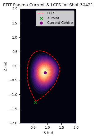
Mirnov Coils#
Mirnov coils are primarily used to measure magnetic fluctuations in the plasma. These fluctuations can provide important information about various plasma instabilities.
They are particularly useful for studying magnetohydrodynamic (MHD) phenomena. MHD activity includes various modes of instabilities, such as kink modes and tearing modes, which can affect plasma confinement and stability.
dataset = xr.open_zarr(
    "https://s3.echo.stfc.ac.uk/mast/level1/shots/29790.zarr", group="xmo"
)
dataset
<xarray.Dataset> Size: 101MB
Dimensions:                        (dim_0: 16, dim_1: 2, time: 1400000)
Coordinates:
  * dim_0                          (dim_0) int32 64B 0 1 2 3 4 ... 12 13 14 15
  * dim_1                          (dim_1) int32 8B 0 1
  * time                           (time) float64 11MB -0.1 -0.1 ... 0.6 0.6
Data variables: (12/18)
    devices_d3_acq216_025_channel  (dim_0) int32 64B ...
    devices_d3_acq216_025_range    (dim_0, dim_1) float32 128B ...
    devices_limit                  (dim_0) float64 128B ...
    omaha_1lz                      (time) float32 6MB ...
    omaha_2lt                      (time) float32 6MB ...
    omaha_2lz                      (time) float32 6MB ...
    ...                             ...
    omaha_5lz                      (time) float32 6MB ...
    omaha_5ur                      (time) float32 6MB ...
    omaha_5ut                      (time) float32 6MB ...
    omaha_5uz                      (time) float32 6MB ...
    omaha_6lz                      (time) float32 6MB ...
    time1                          (time) float64 11MB ...
Attributes:
    description:  Magnetic Field Measurements: OMAHA high frequency Mirnov co...
    file_name:    xmo029790.nc
    format:       CDF
    mds_name:     None
    name:         xmo
    quality:      Not Checked
    shot_id:      29790
    signal_type:  Raw
    source:       xmo
    uda_name:     XMO
    uuid:         ff541ac3-6b1c-5373-8d33-b85fd46bc75b
version: -1- dim_0: 16
- dim_1: 2
- time: 1400000
- dim_0(dim_0)int320 1 2 3 4 5 6 ... 10 11 12 13 14 15
- units :
array([ 0, 1, 2, 3, 4, 5, 6, 7, 8, 9, 10, 11, 12, 13, 14, 15], dtype=int32) - dim_1(dim_1)int320 1
- units :
array([0, 1], dtype=int32)
- time(time)float64-0.1 -0.1 -0.1 -0.1 ... 0.6 0.6 0.6
- units :
- s
array([-0.1     , -0.099999, -0.099999, ...,  0.599998,  0.599999,  0.599999],
      shape=(1400000,))
- devices_d3_acq216_025_channel(dim_0)int32...
- description :
- dims :
- ['dim_0']
- file_name :
- None
- format :
- None
- label :
- mds_name :
- \TOP.RAW.XMO.DEVICES_D3.ACQ216_025:CHANNEL
- name :
- xmo/devices_d3_acq216_025_channel
- quality :
- Not Checked
- rank :
- 1
- shape :
- [16]
- shot_id :
- 29790
- signal_type :
- Raw
- source :
- xmo
- time_index :
- null
- uda_name :
- /XMO/DEVICES/D3_ACQ216_025/CHANNEL
- units :
- uuid :
- b8dfcfeb-7532-5744-a051-05b03e011a92
- version :
- -1
[16 values with dtype=int32]
- devices_d3_acq216_025_range(dim_0, dim_1)float32...
- description :
- dims :
- ['dim_0', 'dim_1']
- file_name :
- None
- format :
- None
- label :
- /devices/d3_acq216_025/range
- mds_name :
- \TOP.RAW.XMO.DEVICES_D3.ACQ216_025:RANGE
- name :
- xmo/devices_d3_acq216_025_range
- quality :
- Not Checked
- rank :
- 2
- shape :
- [16, 2]
- shot_id :
- 29790
- signal_type :
- Raw
- source :
- xmo
- time_index :
- null
- uda_name :
- /XMO/DEVICES/D3_ACQ216_025/RANGE
- units :
- uuid :
- c25d1fcf-4905-53e5-8ab2-ecbb6ed40216
- version :
- -1
[32 values with dtype=float32]
- devices_limit(dim_0)float64...
- description :
- dims :
- ['dim_0']
- file_name :
- None
- format :
- None
- label :
- mds_name :
- \TOP.RAW.XMO.DEVICES:LIMIT
- name :
- xmo/devices_limit
- quality :
- Not Checked
- rank :
- 1
- shape :
- [2]
- shot_id :
- 29790
- signal_type :
- Raw
- source :
- xmo
- time_index :
- null
- uda_name :
- /XMO/DEVICES/LIMIT
- units :
- uuid :
- d1af5b6e-0ba9-51d0-8f62-763cef566a94
- version :
- -1
[16 values with dtype=float64]
- omaha_1lz(time)float32...
- description :
- dims :
- ['time']
- file_name :
- None
- format :
- None
- label :
- arb
- mds_name :
- name :
- xmo/omaha_1lz
- quality :
- Not Checked
- rank :
- 1
- shape :
- [1400000]
- shot_id :
- 29790
- signal_type :
- Raw
- source :
- xmo
- time_index :
- 0
- uda_name :
- /XMO/OMAHA/1LZ
- units :
- uuid :
- ebf41216-9c2f-5910-ad99-ab76b6d2cc3b
- version :
- -1
[1400000 values with dtype=float32]
- omaha_2lt(time)float32...
- description :
- dims :
- ['time']
- file_name :
- None
- format :
- None
- label :
- arb
- mds_name :
- name :
- xmo/omaha_2lt
- quality :
- Not Checked
- rank :
- 1
- shape :
- [1400000]
- shot_id :
- 29790
- signal_type :
- Raw
- source :
- xmo
- time_index :
- 0
- uda_name :
- /XMO/OMAHA/2LT
- units :
- uuid :
- 1e84a280-d09e-5904-800e-ed6868b7dc0b
- version :
- -1
[1400000 values with dtype=float32]
- omaha_2lz(time)float32...
- description :
- dims :
- ['time']
- file_name :
- None
- format :
- None
- label :
- arb
- mds_name :
- name :
- xmo/omaha_2lz
- quality :
- Not Checked
- rank :
- 1
- shape :
- [1400000]
- shot_id :
- 29790
- signal_type :
- Raw
- source :
- xmo
- time_index :
- 0
- uda_name :
- /XMO/OMAHA/2LZ
- units :
- uuid :
- c3f59da1-9cf1-559f-8fc7-80392de84158
- version :
- -1
[1400000 values with dtype=float32]
- omaha_3lt(time)float32...
- description :
- dims :
- ['time']
- file_name :
- None
- format :
- None
- label :
- arb
- mds_name :
- name :
- xmo/omaha_3lt
- quality :
- Not Checked
- rank :
- 1
- shape :
- [1400000]
- shot_id :
- 29790
- signal_type :
- Raw
- source :
- xmo
- time_index :
- 0
- uda_name :
- /XMO/OMAHA/3LT
- units :
- uuid :
- a8d59196-403f-5fe1-9a38-d34de8754cd1
- version :
- -1
[1400000 values with dtype=float32]
- omaha_3lz(time)float32...
- description :
- dims :
- ['time']
- file_name :
- None
- format :
- None
- label :
- arb
- mds_name :
- name :
- xmo/omaha_3lz
- quality :
- Not Checked
- rank :
- 1
- shape :
- [1400000]
- shot_id :
- 29790
- signal_type :
- Raw
- source :
- xmo
- time_index :
- 0
- uda_name :
- /XMO/OMAHA/3LZ
- units :
- uuid :
- 9b985bf1-ab54-55dc-a75c-fbbdfa450902
- version :
- -1
[1400000 values with dtype=float32]
- omaha_4lr(time)float32...
- description :
- dims :
- ['time']
- file_name :
- None
- format :
- None
- label :
- arb
- mds_name :
- name :
- xmo/omaha_4lr
- quality :
- Not Checked
- rank :
- 1
- shape :
- [1400000]
- shot_id :
- 29790
- signal_type :
- Raw
- source :
- xmo
- time_index :
- 0
- uda_name :
- /XMO/OMAHA/4LR
- units :
- uuid :
- daaec6d8-97e0-59d8-9b75-0ad1fdcd7157
- version :
- -1
[1400000 values with dtype=float32]
- omaha_4lt(time)float32...
- description :
- dims :
- ['time']
- file_name :
- None
- format :
- None
- label :
- arb
- mds_name :
- name :
- xmo/omaha_4lt
- quality :
- Not Checked
- rank :
- 1
- shape :
- [1400000]
- shot_id :
- 29790
- signal_type :
- Raw
- source :
- xmo
- time_index :
- 0
- uda_name :
- /XMO/OMAHA/4LT
- units :
- uuid :
- 3b784696-3355-5c48-b419-905ca44b2228
- version :
- -1
[1400000 values with dtype=float32]
- omaha_4lz(time)float32...
- description :
- dims :
- ['time']
- file_name :
- None
- format :
- None
- label :
- arb
- mds_name :
- name :
- xmo/omaha_4lz
- quality :
- Not Checked
- rank :
- 1
- shape :
- [1400000]
- shot_id :
- 29790
- signal_type :
- Raw
- source :
- xmo
- time_index :
- 0
- uda_name :
- /XMO/OMAHA/4LZ
- units :
- uuid :
- 1827c7c0-d688-51be-aa60-b49f70cdecba
- version :
- -1
[1400000 values with dtype=float32]
- omaha_5lt(time)float32...
- description :
- dims :
- ['time']
- file_name :
- None
- format :
- None
- label :
- arb
- mds_name :
- name :
- xmo/omaha_5lt
- quality :
- Not Checked
- rank :
- 1
- shape :
- [1400000]
- shot_id :
- 29790
- signal_type :
- Raw
- source :
- xmo
- time_index :
- 0
- uda_name :
- /XMO/OMAHA/5LT
- units :
- uuid :
- 3f62be95-c42f-5e5a-bf73-03f6d225b9b6
- version :
- -1
[1400000 values with dtype=float32]
- omaha_5lz(time)float32...
- description :
- dims :
- ['time']
- file_name :
- None
- format :
- None
- label :
- arb
- mds_name :
- name :
- xmo/omaha_5lz
- quality :
- Not Checked
- rank :
- 1
- shape :
- [1400000]
- shot_id :
- 29790
- signal_type :
- Raw
- source :
- xmo
- time_index :
- 0
- uda_name :
- /XMO/OMAHA/5LZ
- units :
- uuid :
- cc482786-87a5-59b6-bba0-f344bb6187c0
- version :
- -1
[1400000 values with dtype=float32]
- omaha_5ur(time)float32...
- description :
- dims :
- ['time']
- file_name :
- None
- format :
- None
- label :
- arb
- mds_name :
- name :
- xmo/omaha_5ur
- quality :
- Not Checked
- rank :
- 1
- shape :
- [1400000]
- shot_id :
- 29790
- signal_type :
- Raw
- source :
- xmo
- time_index :
- 0
- uda_name :
- /XMO/OMAHA/5UR
- units :
- uuid :
- 92ebb676-92e0-5c78-a044-8384b4bf1a72
- version :
- -1
[1400000 values with dtype=float32]
- omaha_5ut(time)float32...
- description :
- dims :
- ['time']
- file_name :
- None
- format :
- None
- label :
- arb
- mds_name :
- name :
- xmo/omaha_5ut
- quality :
- Not Checked
- rank :
- 1
- shape :
- [1400000]
- shot_id :
- 29790
- signal_type :
- Raw
- source :
- xmo
- time_index :
- 0
- uda_name :
- /XMO/OMAHA/5UT
- units :
- uuid :
- 86178cf2-ed01-58d8-8be5-9fa72c183679
- version :
- -1
[1400000 values with dtype=float32]
- omaha_5uz(time)float32...
- description :
- dims :
- ['time']
- file_name :
- None
- format :
- None
- label :
- arb
- mds_name :
- name :
- xmo/omaha_5uz
- quality :
- Not Checked
- rank :
- 1
- shape :
- [1400000]
- shot_id :
- 29790
- signal_type :
- Raw
- source :
- xmo
- time_index :
- 0
- uda_name :
- /XMO/OMAHA/5UZ
- units :
- uuid :
- ba8b5d4f-8e89-58a7-8c2b-3405c5a2a112
- version :
- -1
[1400000 values with dtype=float32]
- omaha_6lz(time)float32...
- description :
- dims :
- ['time']
- file_name :
- None
- format :
- None
- label :
- arb
- mds_name :
- name :
- xmo/omaha_6lz
- quality :
- Not Checked
- rank :
- 1
- shape :
- [1400000]
- shot_id :
- 29790
- signal_type :
- Raw
- source :
- xmo
- time_index :
- 0
- uda_name :
- /XMO/OMAHA/6LZ
- units :
- uuid :
- d91166e7-867c-58a0-a710-ff010bd00f44
- version :
- -1
[1400000 values with dtype=float32]
- time1(time)float64...
- description :
- dims :
- ['time']
- file_name :
- None
- format :
- None
- label :
- Time
- mds_name :
- \TOP.RAW.XMO:TIME1
- name :
- xmo/time1
- quality :
- Not Checked
- rank :
- 1
- shape :
- [1400000]
- shot_id :
- 29790
- signal_type :
- Raw
- source :
- xmo
- time_index :
- 0
- uda_name :
- /XMO/TIME1
- units :
- s
- uuid :
- bfe58a24-e54f-5239-afb0-4c84aedc3006
- version :
- -1
[1400000 values with dtype=float64]
- dim_0PandasIndex
PandasIndex(Index([0, 1, 2, 3, 4, 5, 6, 7, 8, 9, 10, 11, 12, 13, 14, 15], dtype='int32', name='dim_0'))
- dim_1PandasIndex
PandasIndex(Index([0, 1], dtype='int32', name='dim_1'))
- timePandasIndex
PandasIndex(Index([-0.09999999999999998, -0.09999949999999998, -0.09999899999999998,
       -0.09999849999999998, -0.09999799999999998, -0.09999749999999998,
       -0.09999699999999997, -0.09999649999999997, -0.09999599999999997,
       -0.09999549999999997,
       ...
         0.5999949999958225,   0.5999954999958225,   0.5999959999958224,
         0.5999964999958224,   0.5999969999958223,   0.5999974999958223,
         0.5999979999958223,   0.5999984999958222,   0.5999989999958222,
         0.5999994999958221],
      dtype='float64', name='time', length=1400000))
- description :
- Magnetic Field Measurements: OMAHA high frequency Mirnov coils (OMAHA), Centre Column Halo Current
- file_name :
- xmo029790.nc
- format :
- CDF
- mds_name :
- None
- name :
- xmo
- quality :
- Not Checked
- shot_id :
- 29790
- signal_type :
- Raw
- source :
- xmo
- uda_name :
- XMO
- uuid :
- ff541ac3-6b1c-5373-8d33-b85fd46bc75b
- version :
- -1
We can first look at the line profile for one of the Mirnov coils:
fig, ax = plt.subplots(1, 1, figsize=(10, 5))
ax.plot(dataset['time'], dataset['omaha_3lz'])
ax.grid()

ax.grid(alpha=0.3)
ax.set_ylabel('Voltage (V)')
ax.set_xlabel('Time (s)')

plt.tight_layout()
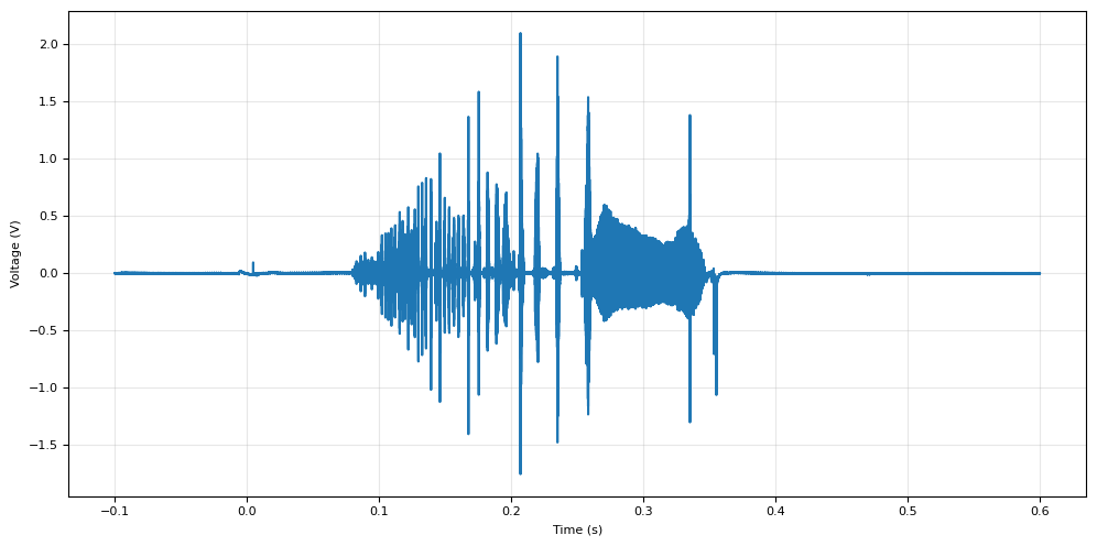
Looking at the spectrogram of the dataset can show us information about the MHD modes. Here we see several mode instabilities occuring before the plasma is lost.
ds = dataset['omaha_3lz']
# Parameters to limit the number of frequencies
nperseg = 2000  # Number of points per segment
nfft = 2000  # Number of FFT points

# Compute the Short-Time Fourier Transform (STFT)
sample_rate = 1/(ds.time[1] - ds.time[0])
f, t, Zxx = stft(ds, fs=int(sample_rate), nperseg=nperseg, nfft=nfft)

fig, ax = plt.subplots(figsize=(15, 5))
cax = ax.pcolormesh(t, f/1000, np.abs(Zxx), shading='nearest', cmap='jet', norm=LogNorm(vmin=1e-5))
ax.set_ylim(0, 50)
ax.set_title(f'XMO/OMAHA/3LZ - Shot {ds.attrs["shot_id"]}')
ax.set_ylabel('Frequency [Hz]')
ax.set_xlabel('Time [sec]')
plt.colorbar(cax, ax=ax)
plt.tight_layout()

Photron Camera Data#
RBA#
RBA contains the data from Photron bullet camera A.
A Photron Bullet Camera provides high-speed, high-resolution imaging of fast transient events in the plasma. Its ability to capture detailed images of plasma instabilities, turbulence, and disruptions makes it essential for understanding and controlling plasma behavior, ultimately aiding in the pursuit of sustained nuclear fusion.
dataset = xr.open_zarr(shot_url, group='rba')
dataset
<xarray.Dataset> Size: 315MB
Dimensions:  (time: 450, height: 912, width: 768)
Coordinates:
  * time     (time) float64 4kB 0.000256 0.002256 0.004256 ... 0.6963 0.6983
Dimensions without coordinates: height, width
Data variables:
    data     (time, height, width) uint8 315MB ...
Attributes: (12/48)
    CLASS:           IMAGE
    IMAGE_SUBCLASS:  IMAGE_INDEXED
    IMAGE_VERSION:   1.2
    board_temp:      0.0
    bottom:          1024
    camera:
    ...              ...
    units:           pixels
    uuid:            f283e185-58a3-54f4-a5f4-a6fef86f9347
    vbin:            0
    version:         -1
    view:            Hl07 floor mount + FFC2 + 25mm lens + CII filter
width: 768- time: 450
- height: 912
- width: 768
- time(time)float640.000256 0.002256 ... 0.6963 0.6983
- units :
- s
array([2.56000e-04, 2.25600e-03, 4.25600e-03, ..., 6.94256e-01, 6.96256e-01,
       6.98256e-01], shape=(450,))
- data(time, height, width)uint8...
[315187200 values with dtype=uint8]
- timePandasIndex
PandasIndex(Index([             0.000256, 0.0022559999999999998,              0.004256,
        0.006255999999999999,              0.008256,              0.010256,
                    0.012256,              0.014256,              0.016256,
        0.018255999999999998,
       ...
                    0.680256,              0.682256,              0.684256,
                    0.686256,              0.688256,              0.690256,
                    0.692256,              0.694256,              0.696256,
                    0.698256],
      dtype='float64', name='time', length=450))
- CLASS :
- IMAGE
- IMAGE_SUBCLASS :
- IMAGE_INDEXED
- IMAGE_VERSION :
- 1.2
- board_temp :
- 0.0
- bottom :
- 1024
- camera :
- ccd_temp :
- 0.0
- codex :
- JP2
- date_time :
- 2013-09-25T13:21:08Z
- depth :
- 8
- description :
- Photron bullet camera A
- dims :
- ['time', 'height', 'width']
- exposure :
- 250.0
- file_format :
- IPX-1
- file_name :
- rba030421.ipx
- filter :
- format :
- IPX
- gain :
- [4.0, 0.0]
- hbin :
- 0
- height :
- 912
- is_color :
- 0
- left :
- 129
- lens :
- mds_name :
- None
- n_frames :
- 450
- name :
- rba
- offset :
- [0.0, 0.0]
- orientation :
- 0
- pre_exp :
- 0.0
- quality :
- Not Checked
- rank :
- 3
- right :
- 896
- shape :
- [450, 912, 768]
- shot :
- 30421
- shot_id :
- 30421
- signal_type :
- Image
- source :
- rba
- strobe :
- 0
- taps :
- 0
- top :
- 113
- trigger :
- -0.10000000149011612
- uda_name :
- RBA
- units :
- pixels
- uuid :
- f283e185-58a3-54f4-a5f4-a6fef86f9347
- vbin :
- 0
- version :
- -1
- view :
- Hl07 floor mount + FFC2 + 25mm lens + CII filter
- width :
- 768
plt.imshow(dataset.data[50], cmap='gray')
plt.tight_layout()
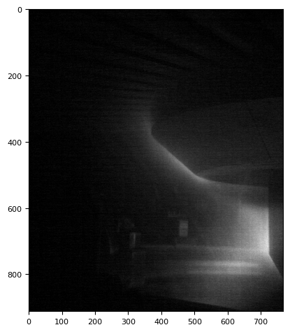
RBB#
RBB contains the data from Photron bullet camera B, which is looking at the central column.
A Photron Bullet Camera provides high-speed, high-resolution imaging of fast transient events in the plasma. Its ability to capture detailed images of plasma instabilities, turbulence, and disruptions makes it essential for understanding and controlling plasma behavior, ultimately aiding in the pursuit of sustained nuclear fusion.
dataset = xr.open_zarr(shot_url, group='rbb')
dataset
<xarray.Dataset> Size: 143MB
Dimensions:  (time: 500, height: 448, width: 640)
Coordinates:
  * time     (time) float64 4kB 1.6e-05 0.002016 0.004016 ... 0.694 0.696 0.698
Dimensions without coordinates: height, width
Data variables:
    data     (time, height, width) uint8 143MB ...
Attributes: (12/48)
    CLASS:           IMAGE
    IMAGE_SUBCLASS:  IMAGE_INDEXED
    IMAGE_VERSION:   1.2
    board_temp:      0.0
    bottom:          680
    camera:
    ...              ...
    units:           pixels
    uuid:            857f64f0-5329-5fc3-9e70-dafd4a69d4e7
    vbin:            0
    version:         -1
    view:            photron HM10 + Dalpha filter
width: 640- time: 500
- height: 448
- width: 640
- time(time)float641.6e-05 0.002016 ... 0.696 0.698
- units :
- s
array([1.60000e-05, 2.01600e-03, 4.01600e-03, ..., 6.94016e-01, 6.96016e-01,
       6.98016e-01], shape=(500,))
- data(time, height, width)uint8...
[143360000 values with dtype=uint8]
- timePandasIndex
PandasIndex(Index([             1.6e-05,             0.002016,             0.004016,
                   0.006016, 0.008015999999999999, 0.010015999999999999,
       0.012015999999999999, 0.014015999999999999,             0.016016,
                   0.018016,
       ...
                   0.680016,             0.682016,             0.684016,
                   0.686016,             0.688016,             0.690016,
                   0.692016,             0.694016,             0.696016,
                   0.698016],
      dtype='float64', name='time', length=500))
- CLASS :
- IMAGE
- IMAGE_SUBCLASS :
- IMAGE_INDEXED
- IMAGE_VERSION :
- 1.2
- board_temp :
- 0.0
- bottom :
- 680
- camera :
- ccd_temp :
- 0.0
- codex :
- JP2
- date_time :
- 2013-09-25T13:06:11Z
- depth :
- 8
- description :
- Photron bullet camera B
- dims :
- ['time', 'height', 'width']
- exposure :
- 10.0
- file_format :
- IPX-1
- file_name :
- rbb030421.ipx
- filter :
- format :
- IPX
- gain :
- [4.0, 0.0]
- hbin :
- 0
- height :
- 448
- is_color :
- 0
- left :
- 193
- lens :
- mds_name :
- None
- n_frames :
- 500
- name :
- rbb
- offset :
- [0.0, 0.0]
- orientation :
- 0
- pre_exp :
- 0.0
- quality :
- Not Checked
- rank :
- 3
- right :
- 832
- shape :
- [500, 448, 640]
- shot :
- 30421
- shot_id :
- 30421
- signal_type :
- Image
- source :
- rbb
- strobe :
- 0
- taps :
- 0
- top :
- 233
- trigger :
- -0.10000000149011612
- uda_name :
- RBB
- units :
- pixels
- uuid :
- 857f64f0-5329-5fc3-9e70-dafd4a69d4e7
- vbin :
- 0
- version :
- -1
- view :
- photron HM10 + Dalpha filter
- width :
- 640
plt.imshow(dataset.data[50], cmap='gray')
plt.tight_layout()